Canonical Correlation simple correlation -- y 1 = x 1

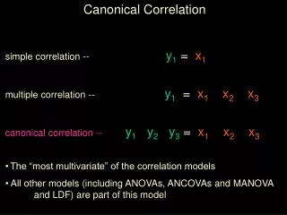
1. Canonical Correlation • simple correlation -- y1 = x1 • multiple correlation -- y1 = x1 x2 x3 • canonical correlation --y1 y2 y3 = x1 x2 x3 • The “most multivariate” of the correlation models • All other models (including ANOVAs, ANCOVAs and MANOVA and LDF) are part of this model

2. Uses and Alternatives for Canonical Correlation • Just because there are multiple criterion variables and multiple predictors doesn’t mean that a canonical correlation is the best analysis for the data! • If your research hypotheses/questions are about correlations between specific criterion variables and specific predictor variables ... • use the specified set of Pearson’s correlations • use Hotelling’s t or Rosenthal’s Z to test hypotheses about which correlations are larger than others (which predictors are more correlated with which criterion variables) • If your research hypotheses/questions are about differences between the best models to understand/predict specific criterion variables • build the specified set of multiple regression models • use “cross-validation” procedures and Hotelling’s/Rosenthal’s tests to compare multiple regression models across the criterion variables

3. Let’s take a look at how canonical correlation “works”, to help understand when to use it (instead of simple or multiple reg)… • Start with multiple y and x variables • y1 y2 y3 = x1 x2 x3 • construct a “canonical variate” as the combination of y variables • CVy1 = b1 y1 + b2 y2 + b3 y3 • construct a “canonical variate” as the combination of x variables • CVx1 = b1 x1 + b2 x2 + b3 x3 • The canonical correlation is the correlation of the canonical variates • Rc = rcvy1, cvx1

4. 1st thing -- The weights used to construct CVy1 and CVx1 are chosen to produce the largest possible Rc • This is different from simple correlation • weighting for X1 is chosen so y’ mimics y • This is different from multiple correlation • weighting for x1 , x2 , etc chosen to maximize the correlation of y’ with y • In canonical correlation the weightings for the Y variables and for the X variables are chosen simultaneously to maximize the correlation between the constructed X variate and the constructed Y variate • 2nd thing -- There can be multiple canonicals • max # is the smaller of the number of criterion & number of predictors • like ldf, have to decide if we have a concentrated or diffuse structure

5. So, canonical correlation is used (instead of comparisons among selected simple and/or multiple correlations) when … • research questions are about which combination(s) of criterion variables are related to which combination(s) or predictors • research questions are about whether the set of variables have a concentrated or a diffuse correlational structure • Examples: • have a set of interrelated criterion variables (e.g., five measures of depression) and want to know if they all share the same relationship with the predictors (a concentrated structure) • have two sets of predictor variables and want to show that one set is most useful for one understanding the one criterion variable and the other set is most useful for understanding a different set of criterion variables

6. Steps of inspecting and describing a canonical correlation… • Determine the number of canonical variates and correlations • maximum number is smaller of # predictors or # criterion • each Rc is tested for H0: Rc = 0 (same test as for MR) • Evaluate the strength of each canonical relationship • Rc² is “shared variance” between that x and y variate • Interpret each canonical variate • Structure weights tell which variables related to which variates • Standardized regression weights tell about the unique contribution of variables to variates

7. Depicting and Describing “Shared Variance” in Canonical Correlation • There are 3 kinds of “shared variances” in cancorr: • RC² • squared canonical correlation • variance shared between the corresponding Y and X canonical variates at • PC • variance shared between a canonical variate and the set of variables from which it is constructed • an index of how well that canonical variate “represents” the set of variables • PC is computed as the average structure weight for that canonical variate • RC • redundancy coefficient • variance shared between a canonical variate from one set of variables and the other set of variables • an index of how well a canonical variate “represents” the other set of variables

8. We start with dependent (y) variables and covariate/predictor (x) variables • a canonical variate is constructed for each set so that the variates are as highly correlated as possible • the RC² tells the variance shared between the canonical variates • the PC tells the variance shared between each canonical variate and the variables from which it was constructed X1 x2 x3 x4 y1 y2 y3 PCx1 PCy1 CVy1 = b1y1 + b2y2 + b3y3 + a CVx1= b1x1 + b2x2 + b3x3 + b4x4 + a RC²

9. We can also ask how much variance is shared between the CV of one set of variables (the covariate/predictor variables) and the other set of variables (the dependent variables)-- a redundancy coefficient • shown is “how much variance among the dependent variables (Ys) is accounted for by the covariate/predictor canonical variate (CVx1) • a redundancy coefficient is calculated as RC² *PC of the variables involved (RC² *PCy1 , here) X1 x2 x3 x4 y1 y2 y3 PCx1 PCy1 redundancy coef. CVx1 CVy1 RC²

10. About the size of the redundancy coefficient • the “old” story was that a small redundancy coefficient meant the canonical correlation analysis was uninteresting or misleading • the “new” story a redundancy coefficient can be “small” for two different reasons that have very different interpretations • “good” -- the CV is “strongly” composed of a minority of the variables in that set (few vars, but with large weights) • often denotes specificity among the variables -- a prerequisite for a diffuse structure • “yucky” -- the CV is “weakly” composed of a majority of the variables in that set (many variables, but small weights) • often denotes that the construct related to the “other vars” is not well-represented by these vars, and so must be “put together” using small portions of ` many vars