Download

1 / 61
610 likes | 742 Vues
Coupling of Atmospheric and Hydrologic Models: A Hydrologic Modeler’s Perspective. George H. Leavesley 1 , Lauren E. Hay 1 , Martyn P. Clark 2 , William J. Gutowski, Jr. 3 , and Robert. L. Wilby 4. 1 U.S. Geological Survey, Denver, CO 2 University of Colorado, Boulder, CO

E N D
Coupling of Atmospheric and Hydrologic Models:A Hydrologic Modeler’s Perspective George H. Leavesley1, Lauren E. Hay1, Martyn P. Clark2, William J. Gutowski, Jr.3, and Robert. L. Wilby4 1U.S. Geological Survey, Denver, CO 2University of Colorado, Boulder, CO 3Iowa State University, Ames, IA 4King’s College London, London, UK
Topics • Water resources issues • Hydrologic modeling approaches • Spatial and temporal distribution issues • Hydrologic forecasting methodologies • Downscaling approaches and applications
Water Resources Simulation and Forecast Needs • Long-term Policy and Planning (10’s of years) • Annual to Inter-annual Operational Planning (6 - 24 months) • Short-term Operational Planning (1 - 30 days) • Flash flood forecasting (hours) • Land-use change and climate variability
SPATIAL CONSIDERATIONS LUMPED MODELS - No account of spatial variability of processes, input, boundary conditions, and system geometry DISTRIBUTED MODELS - Explicit account of spatial variability of processes, input, boundary conditions, and watershed characteristics QUASI-DISTRIBUTED MODELS - Attempt to account for spatial variability, but use some degree of lumping in one or more of the modeled characteristics.
Precipitation and Temperature Distribution Methodologies • Elevation adjustments • Thiessan polygons • Inverse distance weighting • Geostatistical techniques • XYZ method • …
XYZ Methodology Monthly Multiple Linear Regression (MLR) equations developed for PRCP, TMAX, and TMIN using the predictor variables of station location (X, Y) and elevation (Z).
XYZ Spatial Redistribution of Precipitation & Temperature 1. Develop Multiple Linear Regression (MLR) equations (in XYZ) for PRCP, TMAX, and TMIN by month using all appropriate regional observation stations. San Juan Basin Observation Stations 37
Precipitation and temperature stations XYZ Spatial Redistribution 2. Daily mean PRCP, TMAX, and TMIN computed for a subset of stations (3) determined by the Exhaustive Search analysis to be best stations 3. Daily station means from (2) used with monthly MLR xyz relations to estimate daily PRCP, TMAX, and TMIN on each HRU according to the XYZ of each HRU
Plot mean station elevation (Z) vs. mean station PRCP XYZ Methodology • One predictor (Z) example for distributing daily PRCP from a set of stations: • For each day solve for y-intercept • intercept = PRCPsta - slope*Zsta • where PRCPsta is mean station PRCP and • Zsta is mean station elevation • slope is monthly value from MLRs PRCP x Z Slope from monthly MLR used to find the y-intercept 2. PRCPmru = slope*Zmru + intercept where PRCPmru is PRCP for your modeling response unit Zmru is mean elevation of your modeling response unit
XYZ DISTRIBUTION EXHAUSTIVE SEARCH ANALYSIS • Select best station subset from all stations • Estimate gauge undercatch error for • snow events (Bias in observed data) • Select precipitation frequency station set (Bias in observed data)
Forecast Methodologies • - Historic data as analog for the future • Ensemble Streamflow Prediction (ESP) • Synthetic time-series • Weather Generator • - Atmospheric model output • Dynamical Downscaling • Statistical Downscaling
Animas River @ Durango Measured Simulated
Animas Basin Snow-covered Area Year 2000 Simulated Measured (MODIS Satellite) Error Range <= 0.1
ESP – Animas River @ Durango Probability of Exceedance (Frequency Analysis on Peak Flows)
Forecast 4/2/05 Observed 4/3 – 6/30/05 ESP – Animas River @ Durango
Representative Elevation of Atmospheric ModelOutput based on Regional StationObservations Elevation-based Bias Correction
Performance Measures Coefficient of Efficiency E Widely used in hydrology Range – infinity to +1.0 Overly sensitive to extreme values Nash and Sutcliffe, 1970, J. of Hydrology
Nash-Sutcliff Coefficient of Efficiency Scores Simulated vs Observed Daily Streamflow Animas River, Colorado USA
Statistical vs Dynamical Downscaling
Global-scale model National Centers for Environmental Prediction/National Center for Atmospheric Research Reanalysis NCEP
210 km grid spacing Retroactive 51 year record Every 5 days there is an 8-day forecast NCEP
Compare SDS and DDS output by using it to drive the distributed hydrologic model PRMS in 4 basins (DAY 0)
Snowmelt Dominated 526 km2 Cle Elum East Fork of the Carson Rainfall Dominated 3626 km2 Snowmelt Dominated 1792 km2 Animas Snowmelt Dominated 922 km2 Alapaha Study Basins
Cle Elum 500km Buffer radius Alapaha Carson Animas NCEP Grid nodes Basins Statistical Downscaling
Dynamical Downscaling Regional Climate Model – RegCM2 nested within NCEP 52 km grid node spacing 10 year run
Cle Elum East Fork of the Carson Animas Alapaha Dynamical Downscaling
Dynamical Downscaling Animas River Basin RegCM2 grid nodes Buffer Use grid-nodes that fall within 52km buffered area 52 km
Input Data Sets used in Hydrologic Model • Station Data • - BEST-STA • Stations used to calibrate the hydrologic model Climate Stations
Input Data Sets used in Hydrologic Model • Station Data • - BEST-STA - ALL-STA All stations within the RegCM2 buffered area (excluding BEST-STA) Climate Stations
Input Data Sets used in Hydrologic Model • Station Data • - BEST-STA - ALL-STA 2. DDS RegCM2 Grid Nodes
NCEP Grid Nodes Input Data Sets used in Hydrologic Model • Station Data • - BEST-STA - ALL-STA 2. DDS 3. SDS
NCEP Grid Nodes Input Data Sets used in Hydrologic Model • Station Data • - BEST-STA - ALL-STA 2. DDS 3. SDS 4. NCEP
Nash-Sutcliffe Goodness of Fit Statistic Computed between measured and simulated runoff Best-Sta
Nash-Sutcliffe Goodness of Fit Statistic Computed between measured and simulated runoff Best-Sta
Nash-Sutcliffe Goodness of Fit Statistic Computed between measured and simulated runoff Best-Sta INPUT TIME SERIES: Test1 Best-Sta PRCP Bias-DDS TMAX Bias-DDS TMIN Test2 Bias-DDS PRCP Best-Sta TMAX Bias-DDS TMIN Test3 Bias-DDS PRCP Bias-DDS TMAX Best-Sta TMIN
MinimumTemperature Precipitation Maximum Temperature Alapaha Animas Carson Cle Elum R-Square R-Square R-Square SDS SDS SDS DDS DDS DDS All-Sta All-Sta All-Sta NCEP NCEP NCEP Bias-All Bias-All Bias-All Bias-DDS Bias-DDS Bias-DDS Bias-NCEP Bias-NCEP Bias-NCEP R-Square Values between Daily “Best” timeseries and: All-Sta, Bias-All, DDS, Bias-DDS, NCEP, Bias-NCEP, and SDS
MinimumTemperature Precipitation Maximum Temperature Alapaha Animas Carson Cle Elum R-Square R-Square R-Square SDS SDS SDS DDS DDS DDS All-Sta All-Sta All-Sta NCEP NCEP NCEP Bias-All Bias-All Bias-All Bias-DDS Bias-DDS Bias-DDS Bias-NCEP Bias-NCEP Bias-NCEP Snowmelt-dominated basins – highly controlled by daily variations in temperature and radiation Rainfall-dominated basin – highly controlled by daily variations in precipitation
Compare SDS and ESP Forecasts using PRMS Perfect model scenario • Ranked Probability Score • measure of probabilistic forecast skill • forecasts are increasingly penalized as more probability is assigned to event categories further removed from the actual outcome • Ensemble Spread • Range in forecasts
RPSS 0.1 0.3 0.5 0.7 0.9 8 6 4 2 0 8 6 4 2 0 Forecast Day J F M A M J J A S O N D J F M A M J J A S O N D Month Month Ranked Probability Skill Score (RPSS) for forecast days 0-8 and month using measured runoff and simulated runoff produced using: (1)SDSoutput and (2)ESPtechnique Perfect Forecast: RPSS=1 ESP SDS
Forecast Spread for forecast days 0-8 and month using measured runoff and simulated runoff produced using: (1)SDSoutput and (2)ESPtechnique Forecast Spread 500 1500 2500 3500 4500 8 6 4 2 0 8 6 4 2 0 Forecast Day J F M A M J J A S O N D J F M A M J J A S O N D Month Month ESP SDS
Daily basin precipitation mean by month and forecast day for ESP (red line) and SDS (boxplot) R-square values calculated between daily basin-mean measured and (1) SDS and (2) ESP precipitation values Pearson Correlation 0.1 0.2 0.3 0.4 0.5 8 6 4 2 0 8 6 4 2 0 ESP SDS Forecast Day J F M A M J J A S O N D J F M A M J J A S O N D Month Month Comparison of hydrologic model inputs -- Precipitation
Daily basin maximum temperature mean by month and forecast day for ESP (red line) and SDS (boxplot) R-square values calculated between daily basin-mean measured and (1) SDS and (2) ESP maximum temperature values Pearson Correlation 0.1 0.3 0.5 0.7 0.9 8 6 4 2 0 8 6 4 2 0 ESP SDS Forecast Day J F M A M J J A S O N D J F M A M J J A S O N D Month Month Comparison of hydrologic model inputs – Maximum Temperature