Parallel vs Sequential Algorithms
Parallel vs Sequential Algorithms. Design of efficient algorithms. A parallel computer is of little use unless efficient parallel algorithms are available. The issue in designing parallel algorithms are very different from those in designing their sequential counterparts.

Parallel vs Sequential Algorithms
E N D
Presentation Transcript
Design of efficient algorithms A parallel computer is of little use unless efficient parallel algorithms are available. • The issue in designing parallel algorithms are very different from those in designing their sequential counterparts. • A significant amount of work is being done to develop efficient parallel algorithms for a variety of parallel architectures.
Processor Trends • Moore’s Law • performance doubles every 18 months • Parallelization within processors • pipelining • multiple pipelines
Why Parallel Computing • Practical: • Moore’s Law cannot hold forever • Problems must be solved immediately • Cost-effectiveness • Scalability • Theoretical: • challenging problems
Efficient and optimal parallel algorithms • A parallel algorithm is efficient iff • it is fast (e.g. polynomial time) and • the product of the parallel time and number of processors is close to the time of at the best know sequential algorithm T sequential T parallel N processors • A parallel algorithms is optimal iff this product is of the same order as the best known sequential time
The main open question • The basic parallel complexity class is NC. • NC is a class of problems computable in poly-logarithmic time (log c n, for a constant c) using a polynomial number of processors. • P is a class of problems computable sequentially in a polynomial time The main open question in parallel computations is NC = P ?
PRAM 1 2 P1 3 • PRAM - Parallel Random Access Machine • Shared-memory multiprocessor • unlimited number of processors, each • has unlimited local memory • knows its ID • able to access the shared memory in constant time • unlimited shared memory P2 . . . Pi . . Pn m • A very reasonable question: Why do we need a PRAM model? • to make it easy to reason about algorithms • to achieve complexity bounds • to analyze the maximum parallelism
PRAM MODEL 1 2 P1 3 P2 Common Memory . ? . . Pi . . Pn m • PRAM n RAM processors connected to a common memory of m cells • ASSUMPTION: at each time unit each Pican read a memory cell, make an internal • computation and write another memory cell. • CONSEQUENCE:any pair of processor Pi Pjcan communicate in constant time! • Piwrites the message in cell x at timet • Pireads the message in cell x at timet+1
Summary of assumptions for PRAM PRAM • Inputs/Outputs are placed in the shared memory (designated address) • Memory cell stores an arbitrarily large integer • Each instruction takes unit time • Instructions are synchronized across the processors PRAM Instruction Set • accumulator architecture • memory cell R0 accumulates results • multiply/divide instructions take only constant operands • prevents generating exponentially large numbers in polynomial time
PRAM Complexity Measures • for each individual processor • time: number of instructions executed • space: number of memory cells accessed • PRAM machine • time: time taken by the longest running processor • hardware: maximum number of active processors
Two Technical Issues for PRAM • How processors are activated • How shared memory is accessed
Processor Activation • P0 places the number of processors (p) in the designated shared-memory cell • each active Pi, where i < p, starts executing • O(1) time to activate • all processors halt when P0 halts • Active processors explicitly activate additional processors via FORK instructions • tree-like activation • O(log p) time to activate p ... 1 0 0 0 0 0 0 i processor will activate a processor 2i and a processor 2i+1
PRAM • Too many interconnections gives problems with synchronization • However it is the best conceptual model for designing efficient parallel algorithms • due to simplicity and possibility of simulating efficiently PRAM algorithms on more realistic parallel architectures Basic parallel statement for all x in X do in parallel instruction (x) For each x PRAM will assign a processor which will execute instruction(x)
Shared-Memory Access Concurrent (C) means, many processors can do the operation simultaneously in the same memory Exclusive (E) not concurent • EREW (Exclusive Read Exclusive Write) • CREW (Concurrent Read Exclusive Write) • Many processors can read simultaneously the same location, but only one can attempt to write to a given location • ERCW (Exclusive Read Concurrent Write) • CRCW (Concurrent Read Concurrent Write) • Many processors can write/read at/from the same memory location
Concurrent Write (CW) • What value gets written finally? • Priority CW – processors have priority based on which write value is decided • Common CW – multiple processors can simultaneously write only if values are the same • Arbitrary/Random CW – any one of the values are randomly chosen
Example CRCW-PRAM • Initially • table A contains values 0 and 1 • output contains value 0 • The program computes the “Boolean OR” of A[1], A[2], A[3], A[4], A[5]
Example CREW-PRAM • Assume initially table A contains [0,0,0,0,0,1] and we have the parallel program
Pascal triangle PRAM CREW
Membership problem • p processors PRAM with n numbers (p ≤ n) • Does x exist within the n numbers? • P0 contains x and finally P0 has to know Algorithm step1: Inform everyone what x is step2: Every processor checks [n/p] numbers and sets a flag step3: Check if any of the flags are set to 1
One more time about PRAM model • N synchronized processors • Shared memory • EREW, ERCW, • CREW, CRCW • Constant time • access to the memory • standard multiplication/addition • Communication (implemented via access to shared memory)
Two problems for PRAM Problem 1. Min of n numbers Problem 2. Computing a position of the first one in the sequence of 0’s and 1’s. How fast we can compute with many processor and how to reduce the number of processors?
Min of n numbers • Input: Given an array A with n numbers • Output: the minimal number in an array A Optimal Par.Cost = O(n) ? Sequential algorithm Cost = 1 n … Sequential vs. Parallel At least n comparisons should be performed!!! COST = (num. of processors) (time)
Mission: Impossible …computing in a constant time • Archimedes: Give me a lever long enough and a place to stand and I will move the earth • NOWDAYS…. Give me a parallel machine with enough processors and I will find the smallest number in any giant set in a constant time!
Parallel solution 1Min of n numbers • Comparisons between numbers can be done independently • The second part is to find the result using concurrent write mode • For n numbers ----> we have ~ n2 pairs [a1,a2,a3,a4] (a3, a4) (ai ,aj) (a1, a3) (a2, a4) (a1,a2) (a1, a4) n (a2, a3) i j 1 000000000000000000000000000000000000000000000000 1 0 M[1..n] If ai > aj then ai cannot be the minimal number
The following program computes MIN of n numbers stored in the array C[1..n] in O(1) time with n2 processors. Algorithm A1 for each 1 i n do in parallel M[i]:=0 for each 1 i,j n do in parallel if ij C[i] C[j] then M[j]:=1 for each 1 i n do in parallel if M[i]=0 then output:=i
From n2 processors to n1+1/2 Step 1: Partition into disjoint blocks of size Step 2: Apply A1 to each block Step 3: Apply A1 to the results from the step 2 A1 A1 A1 A1 A1 A1 A1 A1 A1 A1 A1
From n1+1/2 processors to n1+1/4 Step 1: Partition into disjoint blocks of size Step 2: Apply A2 to each block Step 3: Apply A2 to the results from the step 2 A2 A2 A2 A2 A2 A2 A2 A2 A2 A2 A2
n2 -> n1+1/2 -> n1+1/4 -> n1+1/8 -> n1+1/16 ->… -> n1+1/k ~ n1 • Assume that we have an algorithm Ak working in O(1) time with processors Algorithm Ak+1 1.Let =1/2 2. Partition the input array C of size n into disjoint blocks of size n each 3. Apply in parallel algorithm Ak to each of these blocks 4. Apply algorithm Ak to the array C’ consisting of n/ n minima in the blocks.
Complexity • We can compute minimum of n numbers using CRCW PRAM model in O(log log n) with n processors by applying a strategy of partitioning the input ParCost = n log log n
Mission: Impossible (Part 2) Computing a position of the first one in the sequence of 0’s and 1’s in a constant time. 00101000 000000000000000000000000000000000000000000000000000000000000000000000000000000000000000000000000000000000000000000000000000000000000000000000000000000000000000000000000000000000000000000000000000000000000000000000000000000000000000000000000000000000000000000000000000000000000100000000000000000010000000000000000000000000010000000000000000000000000000000000000000000100000000000000000000000000000000000000000000000000000001000000100000011111111111111110000000000000000000000010000000000000000000000000000000000000000000000000000000000000000000000000000000000000000000000000000000000100000000000010000000000000000000000000000000000000000000000000000000000000000000000000000000000000000000000111111111111111111111111111111000000000000 00000000000000000000000000000000000000000000000000000000000000000000000000000000000000000000000000000000000000000000000000000000000000000000000000000000000000000000000000000000000000000000000000000000000000000000000000000000000000000000000000000000000000000000000000000000000000000000000000000000000000000000000000000000000000000000000000000000000000000000000000000000000000000000000000000000000000000000000000000000000000000000000000000000000000000000000000000000000000000000000000000000000000000000000000000000000000000000000000000000000000000000000000000000000000000000000000000000000000000000000000000000000000000000000000000000000000000000000000000000000000000000000000000000000000000000000000000000000000000000000000000000000000000000000000000000000000000000000000000000000000000000000000000000000000000000000000000000000000000000000000000000000000000000000000000000000000000000000000000000000000000000000000000000000000000000000000000000000000000000000000000000000000000000000000000000000000000000000000000000000000000000000000000000000000000000000000000000000000000000000000000000000000000000000000000000000000000000000000000000000000000000000000000000000000000000000000000100000000000000000000000000000000000000000000000000000000000000000000000000000000000000000000000000000000000000000000000000000000000000000000000000000000000000000000000000000000000000000000000000000000000010000000001000000000000000000000000000000000000000000000000000000010000000000000000000000000000000000000000000000000000000000000000000000000000000000000000000000000000000000000000000000000000000000000000000000000000000000000000000000000000000000000000000000000000000000000000000000000000000000000000000000000000000000000000000000000000000000000000000000000000000000000000000000000000000000000000000000000000000000000000000000000000000000000000000000000000000000000000000000000000000000000000000000000000000000000000000000000000000000000000000000000000000000000000000000000000000000000000000000000000000000000000000000000000000000000000000000000000000000000000000000000000000000000000000000000000000000000000000000000000000000000000000000000000000000000000000000000000000000000000000000000000000000000000000000000000000000000000000000000000000000000000000000000000000000000000000000000000000000000000000000000000000000000000100000011111111111111110000000000000000000000010000000000000000000000000000000000000000000000000000000000000000000000000000000000000000000000000000000000000000000000000000000000000000000000000000000000000000000000000000000000000000000000000000000000000000000000000000000000100000000000000000010000000000000000000000000010000000000000000000000000000000000000000000100000000000000000000000000000000000000000000000000000001000000100000011111111111111110000000000000000000000010000000000000000000000000000000000000000000000000000000000000000000000000000000000000000000000000000000000000000000000000000000000000000000000000000000000011111111111111111111110000000 00000000 00000001 01101000 00010100
Problem 2.Computing a position of the first one in the sequence of 0’s and 1’s. FIRST-ONE-POSITION(C)=4 for the input array C=[0,0,0,1,0,0,0,1,1,1,0,0,0,1] Algorithm A (2 parallel steps and n2 processors) for each 1 i<j n do in parallel if C[i] =1 and C[j]=1 then C[j]:=0 for each 1 i n do in parallel if C[i] =1 then FIRST-ONE-POSITION:=i 1 1 1 0 After the first parallel step C will contain a single element 1
Reducing number of processors Algorithm B – it reports if there is any one in the table. There-is-one:=0 for each 1 i n do in parallel if C[i] =1 then There-is-one:=1 1 1 000000000000000000 1
Now we can merge two algorithms A and B • Partition table C into segments of size • In each segment apply the algorithm B • Find position of the first one in these sequence by applying algorithm A • Apply algorithm A to this single segment and compute the final value B B B B B B B B B B A A
Complexity • We apply an algorithm A twice and each time to the array of length which need only ( )2 = n processors • The time is O(1) and number of processors is n.
P (complexity) • In computational complexity theory, P is the complexity class containing decision problems which can be solved by a deterministic Turing machine using a polynomial amount of computation time, or polynomial time. • P is known to contain many natural problems, including linear programming, calculating the greatest common divisor, and finding a maximum matching. • In 2002, it was shown that the problem of determining if a number is prime is in P.
P-complete class • In complexity theory, the complexity class P-complete is a set of decision problems and is useful in the analysis of which problems can be efficiently solved on parallel computers. • A decision problem is in P-complete if it is complete for P, meaning that it is in P, and that every problem in P can be reduced to it in polylogarithmic time on a parallel computer with a polynomial number of processors. • In other words, a problem A is in P-complete if, for each problem B in P, there are constants c and k such that B can be reduced to A in time O((log n)c) using O(nk) parallel processors.
Motivation • The class P, typically taken to consist of all the "tractable" problems for a sequential computer, contains the class NC, which consists of those problems which can be efficiently solved on a parallel computer. This is because parallel computers can be simulated on a sequential machine. • It is not known whether NC=P. In other words, it is not known whether there are any tractable problems that are inherently sequential. • Just as it is widely suspected that P does not equal NP, so it is widely suspected that NC does not equal P.
P-complete problems • The most basic P-complete problem is this: Given a Turing machine, an input for that machine, and a number T (written in unary), does that machine halt on that input within the first T steps? • It is clear that this problem is P-complete: if we can parallelize a general simulation of a sequential computer, then we will be able to parallelize any program that runs on that computer. • If this problem is in NC, then so is every other problem in P.
This problem illustrates a common trick in the theory of P-completeness. We aren't really interested in whether a problem can be solved quickly on a parallel machine. • We're just interested in whether a parallel machine solves it much more quickly than a sequential machine. Therefore, we have to reword the problem so that the sequential version is in P. That is why this problem required T to be written in unary. • If a number T is written as a binary number (a string of n ones and zeros, where n=log(T)), then the obvious sequential algorithm can take time 2n. On the other hand, if T is written as a unary number (a string of n ones, where n=T), then it only takes time n. By writing T in unary rather than binary, we have reduced the obvious sequential algorithm from exponential time to linear time. That puts the sequential problem in P. Then, it will be in NC if and only if it is parallelizable.
P-complete problems • Many other problems have been proved to be P-complete, and therefore are widely believed to be inherently sequential. These include the following problems, either as given, or in a decision-problem form: • In order to prove that a given problem is P-complete, one typically tries to reduce a known P-complete problem to the given one, using an efficient parallel algorithm.
Examples of P-complete problems • Circuit Value Problem (CVP) - Given a circuit, the inputs to the circuit, and one gate in the circuit, calculate the output of that gate • Game of Life - Given an initial configuration of Conway's Game of Life, a particular cell, and a time T (in unary), is that cell alive after T steps? • Depth First Search Ordering - Given a graph with fixed ordered adjacency lists, and nodes u and v, is vertex u visited before vertex v in a depth-first search?
Problems not known to be P-complete • Some problems are not known to be either NP-complete or P. These problems (e.g. factoring) are suspected to be difficult. • Similarly there are problems that are not known to be either P-complete or NC, but are thought to be difficult to parallelize. • Examples include the decision problem forms of finding the greatest common divisor of two binary numbers, and determining what answer the extended Euclidean algorithm would return when given two binary numbers.
Conclusion • Just as the class P can be thought of as the tractable problems, so NC can be thought of as the problems that can be efficiently solved on a parallel computer. • NC is a subset of P because parallel computers can be simulated by sequential ones. • It is unknown whether NC = P, but most researchers suspect this to be false, meaning that there are some tractable problems which are probably "inherently sequential" and cannot significantly be sped up by using parallelism • The class P-Complete can be thought of as "probably not parallelizable" or "probably inherently sequential".