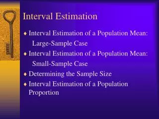

Chapter 9: One- and Two- Sample Estimation
E N D
Presentation Transcript
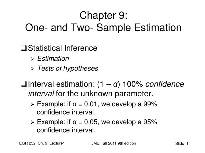
Chapter 9: One- and Two- Sample Estimation • Statistical Inference • Estimation • Tests of hypotheses • Interval estimation: (1 – α) 100% confidence interval for the unknown parameter. • Example: if α = 0.01, we develop a 99% confidence interval. • Example: if α = 0.05, we develop a 95% confidence interval. JMB Fall 2011 9th edition
Single Sample: Estimating the Mean • Given: • σ is known and X is the mean of a random sample of size n, • Then, • the (1 – α)100% confidence interval for μ is 1 - a a/2 a/2 JMB Fall 2011 9th edition
Example A traffic engineer is concerned about the delays at an intersection near a local school. The intersection is equipped with a fully actuated (“demand”) traffic light and there have been complaints that traffic on the main street is subject to unacceptable delays. To develop a benchmark, the traffic engineer randomly samples 25 stop times (in seconds) on a weekend day. The average of these times is found to be 13.2 seconds, and the variance is known to be 4 seconds2. Based on this data, what is the 95% confidence interval (C.I.) around the mean stop time during a weekend day? JMB Fall 2011 9th edition
Example (cont.) X = ______________ σ = _______________ α = ________________ α/2 = _____________ Z0.025 = _____________ Z0.975 = ____________ Solution: 12.416 < μSTOP TIME < 13.984 Z0.025 = -1.96 Z0.975 = 1.96 13.2-(1.96)(2/sqrt(25)) = 12.416 13.2+(1.96)(2/sqrt(25)) = 13.984 JMB Fall 2011 9th edition
Your turn … • What is the 90% C.I.? What does it mean? 90% 5% 5% Z(.05) = + 1.645 All other values remain the same. The 90 % CI for μ = (12.542,13.858) Note that the 95% CI is wider than the 90% CI. JMB Fall 2011 9th edition
What if σ2is unknown? • For example, what if the traffic engineer doesn’t know the variance of this population? • If n is sufficiently large (n > 30), then the large sample confidence intervalis calculated by using the sample standard deviation in place of sigma: • If σ2is unknown and n is not “large”, we must use the t-statistic. JMB Fall 2011 9th edition
Single Sample: Estimating the Mean(σ unknown, n not large) • Given: • σ is unknown and X is the mean of a random sample of size n (where n is not large), • Then, • the (1 – α)100% confidence interval for μ is: JMB Fall 2011 9th edition
Recall Our Example A traffic engineer is concerned about the delays at an intersection near a local school. The intersection is equipped with a fully actuated (“demand”) traffic light and there have been complaints that traffic on the main street is subject to unacceptable delays. To develop a benchmark, the traffic engineer randomly samples 25 stop times (in seconds) on a weekend day. The average of these times is found to be 13.2 seconds, and the sample variance, s2, is found to be 4 seconds2. Based on this data, what is the 95% confidence interval (C.I.) around the mean stop time during a weekend day? JMB Fall 2011 9th edition
Small Sample Example (cont.) n = _______ df = _______ X = ______ s = _______ α = _______ α/2 = ____ t0.025,24 = _______ _______________ < μ < ________________ 13.2 - (2.064)(2/sqrt(25)) = 13.374 13.2 + (2.064)(2/sqrt(25)) = 14.026 JMB Fall 2011 9th edition
Your turn A thermodynamics professor gave a physics pretest to a random sample of 15 students who enrolled in his course at a large state university. The sample mean was found to be 59.81 and the sample standard deviation was 4.94. Find a 99% confidence interval for the mean on this pretest. JMB Fall 2011 9th edition
Solution X = ______________ s = _______________ α = ________________ α/2 = _____________ (draw the picture) t___ , ____ = _____________ __________________ < μ < ___________________ X = 59.81 s = 4.94 α = .01 α/2 = .005 t (.005,14) = 2.977 Lower Bound 59.81 - (2.977)(4.94/sqrt(15)) = 56.01 Upper Bound 59.81 + (2.977)(4.94/sqrt(15)) = 63.61 JMB Fall 2011 9th edition
Standard Error of a Point Estimate • Case 1: σ known • The standard deviation, or standard error of X is • Case 2: σ unknown, sampling from a normal distribution • The standard deviation, or (usually) estimated standard error of X is JMB Fall 2011 9th edition
9.6: Prediction Interval • For a normal distribution of unknown mean μ, and standard deviation σ, a 100(1-α)% prediction interval of a future observation, x0is if σ is known, and if σ is unknown JMB Fall 2011 9th edition
9.7: Tolerance Limits • For a normal distribution of unknown mean μ, and unknown standard deviation σ, tolerance limits are given by x + ks where k is determined so that one can assert with 100(1-γ)% confidence that the given limits contain at least the proportion 1-α of the measurements. • Table A.7 (page 745) gives values of k for (1-α) = 0.9, 0.95, or 0.99 and γ = 0.05 or 0.01 for selected values of n. JMB Fall 2011 9th edition
Case Study 9.1c (Page 281) • Find the 99% tolerance limits that will contain 95% of the metal pieces produced by the machine, given a sample mean diameter of 1.0056 cm and a sample standard deviation of 0.0246. • Table A.7 (page 745) • (1 - α ) = 0.95 • (1 – Ƴ ) = 0.99 • n = 9 • k = 4.550 • x ± ks = 1.0056 ± (4.550) (0.0246) • We can assert with 99% confidence that the tolerance interval from 0.894 to 1.117 cm will contain 95% of the metal pieces produced by the machine. JMB Fall 2011 9th edition
Summary JMB Fall 2011 9th edition