One- and Two-Sample Tests of Hypotheses
290 likes | 553 Vues
One- and Two-Sample Tests of Hypotheses. Chapter 10. 10.1 Statistical Hypotheses. Real life problems are usually different than just estimation of population statistics. We try on the basis of experimental evidence Whether coffee drinking increses the risk of cancer

One- and Two-Sample Tests of Hypotheses
E N D
Presentation Transcript
One- and Two-Sample Tests of Hypotheses Chapter 10
10.1 Statistical Hypotheses • Real life problems are usually different than just estimation of population statistics. • We try on the basis of experimental evidence • Whether coffee drinking increses the risk of cancer • Whether there is difference between the accuracy of two kinds of gauges • Whether a person’s eye color and blood type are independent variables.
Statistical hypotheses • We postulate or conjecture something about the system • In each case, the conjecture can be put in the form of a statistical hypothesis • Defn: • A statistical hypothesis is an assertion or conjecture • Truth is never known unless we examine the entire population.
Accepting hypotheses As always, we take a random sample from the population. Evidence from the sample that is inconsistent with the stated hypothesis leads to a rejection of the hypothesis.
The Role of Probability in Hypothesis Testing Hypothesis: A fraction p = 0.1 of a production is defective Sample of 100 units, 12 defective We cannot refute the claim p=0.1 But we also cannot refute p=0.12 or p=0.15 The rejection of a hypothesis means that the evidence from the sample refutes it.
Rejection of a Hypothesis • Rejection means that there is a small probability of of obtaining the sample information observed when, in fact, the hypothesis is true. • Hypothesis that p=0.1 is unlikely if there are 20 defective units in a sample of 100 units. • Why? • If p=0.1, probability of observing 20 defective units is 0.002 • Rejection rules out the hypothesis, failing to reject, does not. But it does not rule out other hypotheses as well.
Establishing a Conclusion • Rejecting a hypothesis is stronger than failing to reject it. • If you want to show that • Coffee drinking increases the risk of cancer • One gauge is more accurate than another • Your hypothesis should be • “There is no increased cancer risk” • “There is no difference between gauges”
The Null and Alternative Hypotheses • Null hypothesis: • The hypothesis we wish to test, which is denoted by H0 • Alternative hypothesis: • The rejection of H0 leads to acceptance of this hypothesis, denoted by H1 • H1 is the question to be answered, or the theory to be tested, whereas H0 nullifies H1
Arriving conclusions • Reject H0: in favor of H1 because of sufficient evidence in the data • Fail to reject H0: because of insufficient evidence in the data. • We never acceptH0 • For our example: • H0 : p = 0.1 • H1 : p > 0.1
10.2 Testing a Statistical Hypothesis • A certain type of cold vaccine is known to be only 25% effective after a period of 2 years. • We want to determine if a new kind of vaccine is effective for a longer period of time. • Experiment: • Choose 20 people at random and inoculate them with the new vaccine • If more than 8 remain healthy after 2 years, we conclude that the new vaccine is better.
Example (cont.) • In actual situations we need thousands of people • The number 8 seems arbitrary, but reasonable • We are testing the null hypothesis that • The new vaccine is equally effective after 2 years as the former one. • The alternative hypothesis is that • The new vaccine is effective for a longer period of time.
Example (cont.) This is equal to testing the hypothesis that the binomial parameter for the probability of a success on a given trial is p = 0.25, against the alternative that p > 0.25. H0 : p = 0.25 H1: p > 0.25
The Test Statistic • The test statistic is the observed statistic on which we base our decision. • In this case, it is X, the number of healthy people after two years • The values of X that makes us reject the null hypothesis constitute the critical region • The last number we observe before passing into the critical region is the critical value • In this case, it is 8.
Types of Error • This decision procedure could lead to either of two wrong conlusions • Type I error: • Rejecting H0in favor of H1 when, in fact, H0is true. • The probability of a type I error, also called level of significance, is denoted by α. • Type II error: • Failing to reject H0when, in fact, H0is false. • The probability of type II error, denoted by β, is impossible to compute unless we have a specific H1
Possible Situations Type II error cannot be computed without a specific alternative hypothesis.
Computing Type II Error Null hypothesis is p = 0.25 As alternative hypothesis, use a specific value for p, such as 0.5 Then, we get
How to Choose α and β • Ideally, both types of error should be small • For some applications, onw type of error might be more important than the other • How to change α and β ? • Either change the critical value • Usually decreases one type of error while increasing the other • Or change the sample size • Increasing the sample size reduces both types of error
The role of α, β and the Sample Size • In our example • Change critical value from 8 to 7 • αincreases to 0.1018 • β decreases to 0.1316 • Change sample size from 20 to 100 (c.v. 36) • αdecreases to 0.0039 • β decreases to 0.0035 • Read text book pages 326-327 for details • These concepts can be equally well applied to continuous random variables.
Important Properties of a Test of Hypothesis 1- The type I error and type II error are related. A decrease in the probability of one generally results in an increase in the probability of the other 2- The size of the critical region, and therefore the probability of committing a type I error, can always be reduced by adjusting the critical values
Important Properties of a Test of Hypothesis 3- An increase in the sample size will reduce both types of error simultaneously 4- If the null hypothesis is false, β is a maximum when the true value of a parameter approaches the hypothesized value. The greater the distance between the true value and the hypothesized value, the smaller β will be.
The Power of a Test • Definition: • The power of a test is the probability of rejecting H0 given that a specific alternative is true • Which is 1 – β • Different kinds of tests are compared by contrasting power properties. • To increase the power of a test, either increase α, or increase sample size
One- and Two-Tailed Tests • One-tailed test • A test of any hypothesis where the alternative is one sided, such as • H0 : θ = θ0 • H1: θ> θ0 or H1: θ< θ0 where critical region is not split • Two-tailed test • A test of any hypothesis where the alternative is two sided, such as • H0 : θ = θ0 • H1 : θ≠ θ0 where critical region is split into two
Choosing Null and Alternative Hypotheses • Example 10.1 • A manufacturer of a certain brand of rice cereal claims that the average saturated fat content does not exceed 1.5 mg. • State the null and alternative hypotheses to be used in testing this claim and determine where the critical region is located.
Choosing Null and Alternative Hypotheses • Solution • The claim should be rejected only if the average is greater than 1.5 mg and should not be rejected if average is less than or equal to 1.5 mg. • H0 : μ = 1.5mg • H1: μ> 1.5mg - one-tailed • Note that the nonrejection of H0 does not rule out values less than 1.5mg. The critical region lies entirely in the right tail of the distribution.
Choosing Null and Alternative Hypotheses • Example 10.2 • A real estate agent claims that 60% of all private residences being built today are 3-bedroom homes. To test this claim, a large sample of new residences is inspected; the proportion of these homes with 3 bedrooms is recorded and used as our test statistic. • State the null and alternative hypotheses to be used in testing this claim and determine where the critical region is located.
Choosing Null and Alternative Hypotheses • Solution • We reject if the test statistic is significantly higher or lower than p=0.6. • H0 : p = 0.6 • H1 : p ≠ 0.6 • The alternative hypothesis implies a two-tailed test, where the critical region is symetrically split into two.
10.4 The Use of P values for Decision Making • Classical Hypothesis Testing • We usually use a prefixed probability of type I error • 1 – State the null and alternative hypotheses • 2 – Choose a fixed significance level α • 3 – Choose a test statistic and establish a critical region • 4 – Frome the computed test statistic, reject H0 if the test statistic is in the critical region. Otherwise do not reject. • 5 – Draw conclusions
The Problem with Classical Approach Classical approach either rejects or fails to reject. Even if we fail to reject, the risk of rejecting can be very low, if the observed statistic is very close to the critical value. If we only reject using the critical value and the test statistic, we lose important information, namely, how likely it is to observe the data if the null hypothesis is true. This probability is called the P-value.
P-Value • A P-Value is the lowest level (of significance) at which the observed value of the test statistic is significant. • Significance Testing • 1 – State null and alternative hypotheses • 2 – Choose an appropriate test statistic • 3 – Compute P-value based on computed value of test statistic • 4 – Use judgment based on P-value and knowledge of scientific system.