Tests of Hypotheses

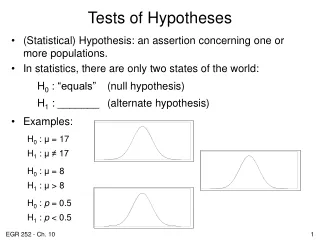
1. Tests of Hypotheses • (Statistical) Hypothesis: an assertion concerning one or more populations. • In statistics, there are only two states of the world: H0 : “equals” (null hypothesis) H1 : _______ (alternate hypothesis) • Examples: H0 : μ = 17 H1 : μ ≠ 17 H0 : μ = 8 H1 : μ > 8 H0 : p = 0.5 H1 : p < 0.5

2. Choosing a Hypothesis • Your turn … Suppose a coffee vending machine claims it dispenses an 8-oz cup of coffee. You have been using the machine for 6 months, but recently it seems the cup isn’t as full as it used to be. You plan to conduct a test of your hypothesis. What are your hypotheses?

3. Level of significance, α Probability of committing a Type I error = P (rejecting H0 | H0 is true) β Probability of committing a Type II error Power of the test = ________ (probability of rejecting the null hypothesis given that the alternate is true.) Hypothesis testing

4. Determining α & β • Example: Proportion of adults in a small town who are college graduates is estimated to be p = 0.6. A random sample of 15 adults is selected to test this hypothesis. If we find that between 6 and 12 adults are college graduates, we will accept H0 : p = 0.6; otherwise we will reject the hypothesis and conclude the proportion is something different (for this example, use H1: p = 0.5). α = ________________ β = ________________

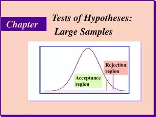
5. Hypothesis Testing • Approach 1 - Fixed probability of Type I error. • State the null and alternative hypotheses. • Choose a fixed significance level α. • Specify the appropriate test statistic and establish the critical region based on α. Draw a graphic representation. • Compute the value of the test statistic based on the sample data. • Make a decision to reject or fail to reject H0, based on the location of the test statistic. • Draw an engineering or scientific conclusion.

6. Approach 2 - Significance testing (P-value approach) State the null and alternative hypotheses. Choose an appropriate test statistic. Compute value of test statistic and determine P-value. Draw conclusion based on P-value. Hypothesis Testing P = 0 P = 1 0.75 0.25 0.5

7. Hypothesis Testing Tells Us … • Strong conclusion: • If our calculated t-value is “outside” tα,ν (approach 1) or we have a small p-value (approach 2), then we reject H0: μ = μ0 in favor of the alternate hypothesis. • Weak conclusion: • If our calculated t-value is “inside” tα,ν (approach 1) or we have a “large” p-value (approach 2), then we cannot reject H0: μ = μ0. • In other words: • Failure to reject H0 does not imply that μ is equal to the stated value, only that we do not have sufficient evidence to favor H1.

8. Single Sample Test of the Mean A sample of 20 cars driven under varying highway conditions achieved fuel efficiencies as follows: Sample mean x = 34.271 mpg Sample std dev s = 2.915 mpg Test the hypothesis that the population mean equals 35.0 mpg vs. μ< 35. H0: ________ n = ________ H1: ________ σ unknown use ___ distribution.

9. Example (cont.) Approach 2: = _________________ Using Excel’s tdist function, P(x ≤ -1.118) = _____________ Conclusion: __________________________________

10. Example (concl.) Approach 1: t0.05,19 = _____________ Since H1 specifies “< μ,” tcrit = ___________ tcalc = _________ Conclusion: _________________________________

11. Your turn … A sample of 20 cars driven under varying highway conditions achieved fuel efficiencies as follows: Sample mean x = 34.271 mpg Sample std dev s = 2.915 mpg Test the hypothesis that the population mean equals 35.0 mpg vs. μ≠ 35 at an α level of 0.05. Draw the picture.

12. Two-Sample Hypothesis Testing • Example: A professor has designed an experiment to test the effect of reading the textbook before attempting to complete a homework assignment. Four students who read the textbook before attempting the homework recorded the following times (in hours) to complete the assignment: 3.1, 2.8, 0.5, 1.9 hours Five students who did not read the textbook before attempting the homework recorded the following times to complete the assignment: 0.9, 1.4, 2.1, 5.3, 4.6 hours

13. Two-Sample Hypothesis Testing • Define the difference in the two means as: μ1 - μ2 = d0 • What are the Hypotheses? H0: _______________ H1: _______________ or H1: _______________ or H1: _______________

14. Our Example Reading: n1 = 4 x1 = 2.075 s12 = 1.363 No reading: n2 = 5 x2 = 2.860 s22 = 3.883 If we assume the population variances are “equal”, we can calculate sp2 and conduct a __________. = __________________

15. Your turn … • Lower-tail test ((μ1 - μ2 < 0) • “Fixed α” approach (“Approach 1”) at α = 0.05 level. • “p-value” approach (“Approach 2”) • Upper-tail test (μ2 – μ1 > 0) • “Fixed α” approach at α = 0.05 level. • “p-value” approach • Two-tailed test (μ1 - μ2 ≠ 0) • “Fixed α” approach at α = 0.05 level. • “p-value” approach Recall 

16. Lower-tail test ((μ1 - μ2 < 0) • Draw the picture: • Solution: • Decision: • Conclusion:

17. Upper-tail test (μ2 – μ1 > 0) • Draw the picture: • Solution: • Decision: • Conclusion:

18. Two-tailed test (μ1 - μ2 ≠ 0) • Draw the picture: • Solution: • Decision: • Conclusion:

19. Another Example Suppose we want to test the difference in carbohydrate content between two “low-carb” meals. Random samples of the two meals are tested in the lab and the carbohydrate content per serving (in grams) is recorded, with the following results: n1 = 15 x1 = 27.2 s12 = 11 n2 = 10 x2 = 23.9 s22 = 23 tcalc = ______________________ ν = ________________ (using equation in table 10.2)

20. Example (cont.) • What are our options for hypotheses? • At an α level of 0.05, • One-tailed test, t0.05, 15 = ________ • Two-tailed test, t0.025, 15 = ________ • How are our conclusions affected?

21. Special Case: Paired Sample T-Test Examples Paired-sample? • Car Radial Belted 1 ** ** Radial, Belted tires 2 ** ** placed on each car. 3 ** ** 4 ** ** • Person Pre Post 1 ** ** Pre- and post-test 2 ** ** administered to each 3 ** ** person. 4 ** ** • Student Test1 Test2 1 ** ** 5 scores from test 1, 2 ** ** 5 scores from test 2. 3 ** ** 4 ** **

22. Example* Nine steel plate girders were subjected to two methods for predicting sheer strength. Partial data are as follows: GirderKarlsruheLehighdifference, d 1 1.186 1.061 2 1.151 0.992 9 1.559 1.052 Conduct a paired-sample t-test at the 0.05 significance level to determine if there is a difference between the two methods. * adapted from Montgomery & Runger, Applied Statistics and Probability for Engineers.

23. Example (cont.) Hypotheses: H0: μD = 0 H1: μD ≠ 0 t__________ = ______ Calculate difference scores (d), mean and standard deviation, and tcalc … d = 0.2736 sd = 0.1356 tcalc = ______________________________

24. What does this mean? • Draw the picture: • Decision: • Conclusion:

25. Goodness-of-Fit Tests • Procedures for confirming or refuting hypotheses about the distributions of random variables. • Hypotheses: H0: The population follows a particular distribution. H1: The population does not follow the distribution. Examples: H0: The data come from a normal distribution. H1: The data do not come from a normal distribution.

26. Goodness of Fit Tests (cont.) • Test statistic is χ2 • Draw the picture • Determine the critical value χ2 with parameters α, ν = k – 1 • Calculate χ2 from the sample • Compare χ2calcto χ2crit • Make a decision about H0 • State your conclusion

27. Tests of Independence • Hypotheses H0: independence H1: not independent • Example Choice of pension plan. 1. Develop a Contingency Table

28. Example 2. Calculate expected probabilities P(#1 ∩ S) = _______________ E(#1 ∩ S) = _____________ P(#1 ∩ H) = _______________ E(#1 ∩ H) = _____________ (etc.)

29. Hypotheses • Define Hypotheses H0: the categories (worker & plan) are independent H1: the categories are not independent 4. Calculate the sample-based statistic = ________________________________________ = ______

30. The Test 5. Compare to the critical statistic, χ2α, r where r = (a – 1)(b – 1) for our example, say α = 0.01 χ2_____ = ___________ Decision: Conclusion:

31. Homework for Thursday, March 23 • 3, 6, 7 (pg. 319) (Refer to your updated schedule for future homework assignments.)