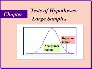
Tests of Hypotheses Based on a Single Sample
430 likes | 563 Vues
This guide provides a detailed overview of hypothesis testing, focusing on evaluating claims about a population mean using a single sample. It covers essential concepts such as null and alternative hypotheses, one-tailed and two-tailed tests, test statistics, and p-values. By understanding how to interpret sample data in the context of probability, readers can make informed decisions about the validity of statistical claims. The significance level (alpha) plays a crucial role in determining whether to reject or fail to reject the null hypothesis, emphasizing the importance of rigorous statistical inference.

Tests of Hypotheses Based on a Single Sample
E N D
Presentation Transcript
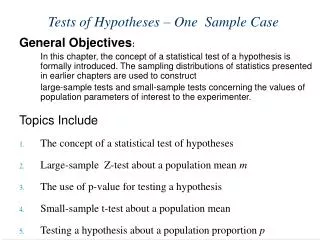
Overview of Inference • Methods for drawing conclusions about a population from sample data are called statistical inference • Methods • Confidence Intervals - estimating a value of a population parameter • Tests of hypotheses - assess evidence for a claim about a population • Inference is appropriate when data are produced by either • a random sample or • a randomized experiment
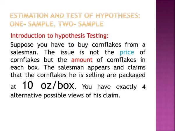
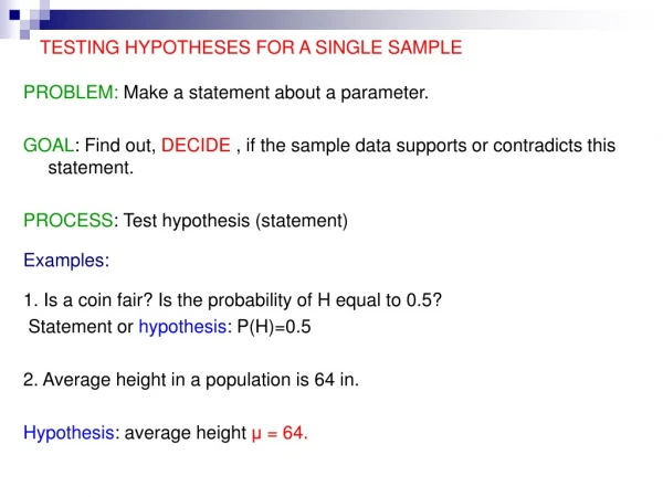
Stating hypotheses A test of hypothesis tests a specific hypothesis using sample data to decide on the validity of the hypothesis. In statistics, a hypothesis is an assumption or a theory about the characteristics of one or more variables in one or more populations. What you want to know: Does the calibrating machine that sorts cherry tomatoes into packs need revision? The same question reframed statistically: Is the population mean µ for the distribution of weights of cherry tomato packages equal to 227 g (i.e., half a pound)?
The null hypothesis is a very specific statement about a parameter of the population(s). It is labeled H0. The alternative hypothesis is a more general statement about a parameter of the population(s) that is exclusive of the null hypothesis. It is labeled Ha. Weight of cherry tomato packs: H0 : µ = 227 g (µis the average weight of the population of packs) Ha : µ ≠ 227 g (µ is either larger or smaller)
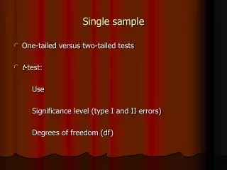
One-sided and two-sided tests • A two-tail or two-sided test of the population mean has these null and alternative hypotheses: H0 : µ= [a specific number] Ha: µ [a specific number] • A one-tail or one-sided test of a population mean has these null and alternative hypotheses: H0 : µ= [a specific number] Ha : µ < [a specific number] OR H0 : µ = [a specific number] Ha : µ > [a specific number] The FDA tests whether a generic drug has an absorption extent similar to the known absorption extent of the brand-name drug it is copying. Higher or lower absorption would both be problematic, thus we test: H0 : µgeneric = µbrandHa : µgenericµbrand two-sided
Test Statistic A test of significance is based on a statistic that estimates the parameter that appears in the hypotheses. When H0 is true, we expect the estimate to take a value near the parameter value specified in H0. Values of the estimate far from the parameter value specified by H0 give evidence against H0. A teststatisticcalculated from the sample data measures how far the data diverge from what we would expect if the null hypothesis H0 were true. Large values of the statistic show that the data are not consistent with H0.
P-Value The null hypothesis H0states the claim that we are seeking evidence against. The probability that measures the strength of the evidence against a null hypothesis is called a P-value. The probability, computed assuming H0is true, that the statistic would take a value as extreme as or more extreme than the one actually observed is called the P-value of the test. The smaller the P-value, the stronger the evidence against H0 provided by the data. • Small P-values are evidence against H0because they say that the observed result is unlikely to occur when H0is true. • Large P-values fail to give convincing evidence against H0because they say that the observed result is likely to occur by chance when H0is true.
Statistical Significance The final step in performing a significance test is to draw a conclusion about the competing claims you were testing. We will make one of two decisions based on the strength of the evidence against the null hypothesis (and in favor of the alternative hypothesis)―reject H0or fail to reject H0. • If our sample result is too unlikely to have happened by chance assuming H0is true, then we’ll reject H0. • Otherwise, we will fail to reject H0. Note:A fail-to-reject H0 decision in a significance test doesn’t mean that H0 is true. For that reason, you should never “accept H0” or use language implying that you believe H0 is true. In a nutshell, our conclusion in a significance test comes down to: P-value small → reject H0→ conclude Ha(in context) P-value large → fail to reject H0→ cannot conclude Ha(in context)
Statistical Significance There is no rule for how small a P-value we should require in order to reject H0— it’s a matter of judgment and depends on the specific circumstances. But we can compare the P-value with a fixed value that we regard as decisive, called the significance level. We write it as , the Greek letter alpha. When our P-value is less than the chosen , we say that the result is statistically significant. If the P-value is smaller than alpha, we say that the data are statistically significant at level . The quantity is called the significance levelor the level of significance. When we use a fixed level of significance to draw a conclusion in a significance test, P-value < → reject H0→ conclude Ha(in context) P-value ≥ → fail to reject H0→ cannot conclude Ha(in context)
Four Steps of Tests of Significance Tests of Significance: Four Steps 1. State the null and alternative hypotheses. 2. Calculate the value of the test statistic. 3. Find the P-value for the observed data. 4. State a conclusion. We will learn the details of many tests of significance in the following chapters. The proper test statistic is determined by the hypotheses and the data collection design.
Does the packaging machine need revision? H0 : µ = 227 g versus Ha : µ ≠ 227 g What is the probability of drawing a random sample such as yours if H0 is true? Sampling distribution σ/√n = 2.5 g 2.28% 2.28% µ (H0) From table A, the area under the standard normal curve to the left of z is 0.0228. Thus, P-value = 2*0.0228 = 4.56%. The probability of getting a random sample average so different fromµ is so low that we reject H0. The machine does need recalibration.
The significance level: a The significance level, α, is the largest P-value tolerated for rejecting a true null hypothesis (how much evidence against H0 we require). This value is decided arbitrarily before conducting the test. • If the P-value is equal to or less than α(P ≤ α), then we reject H0. • If the P-value is greater than α (P > α), then we fail to reject H0. Does the packaging machine need revision? Two-sided test. The P-value is 4.56%. * If α had been set to 5%, then the P-value would be significant. * If α had been set to 1%, then the P-value would not be significant.
Two-Sided Significance Tests and Confidence Intervals Because a two-sided test is symmetrical, you can also use a 1 – a confidence interval to test a two-sided hypothesis at level a. In a two-sided test, C = 1 – C confidence level significance level α /2 α /2
Sweetening colas Cola manufacturers want to test how much the sweetness of a new cola drink is affected by storage. The sweetness loss due to storage was evaluated by 10 professional tasters (by comparing the sweetness before and after storage): Taster Sweetness loss • 1 2.0 • 2 0.4 • 3 0.7 • 4 2.0 • 5 −0.4 • 6 2.2 • 7 −1.3 • 8 1.2 • 9 1.1 • 10 2.3 Obviously, we want to test if storage results in a loss of sweetness, thus: H0: m = 0 versus Ha: m > 0 This looks familiar. However, here we do not know the population parameter s. • The population of all cola drinkers is too large. • Since this is a new cola recipe, we have no population data. This situation is very common with real data.
When the sample size is large, the sample is likely to contain elements representative of the whole population. Then s is a good estimate of s. But when the sample size is small, the sample contains only a few individuals. Then s is a mediocre estimate of s. When s is unknown The sample standard deviation s provides an estimate of the population standard deviation s. Populationdistribution Large sample Small sample
Standard deviation s – standard error s/√n For a sample of size n, the sample standard deviation s is: The value s/√n is called the standard error of the mean .
The t distributions Suppose that an SRS of size n is drawn from an N(µ, σ) population. • When s is known, the sampling distribution is N(m, s/√n). • When s is estimated from the sample standard deviation s, the sampling distribution follows at distribution t(m, s/√n) with degrees of freedom n − 1. is the one-sample t statistic.
When n is very large, s is a very good estimate of s, and the corresponding t distributions are very close to the normal distribution. The t distributions become wider for smaller sample sizes, reflecting the lack of precision in estimating s from s.
Standardizing the data before using t-table As with the normal distribution, the first step is to standardize the data. Then we can use t-table to obtain the area under the curve. t(m,s/√n) df = n − 1 t(0,1)df = n − 1 1 s/√n m t 0
When σ is unknown, we use a t distribution with “n−1” degrees of freedom (df). Table shows the z-values and t-values corresponding to landmark P-values/ confidence levels. When σ is known, we use the normal distribution and the standardized z-value. T-table
t-table gives the area to the RIGHT of a dozen t or z-values. It can be used for t distributions of a given df and for the Normal distribution. (…) z-table vs. t-table Z-table gives the area to the LEFT of hundreds of z-values. It should only be used for Normal distributions. (…) Table D T-table also gives the middle area under a t or normal distribution comprised between the negative and positive value of t or z.
One-sided (one-tailed) Two-sided (two-tailed) The P-value is the probability, if H0 is true, of randomly drawing a sample like the one obtained or more extreme, in the direction of Ha. The P-value is calculated as the corresponding area under the curve, one-tailed or two-tailed depending on Ha:
For df = 9 we only look into the corresponding row. The calculated value of t is 2.7. We find the 2 closest t values. 2.398 < t = 2.7 < 2.821 thus 0.02 > upper tail p > 0.01 T-table For a one-sided Ha, this is the P-value (between 0.01 and 0.02); for a two-sided Ha, the P-value is doubled (between 0.02 and 0.04).
Sweetening colas (continued) Is there evidence that storage results in sweetness loss for the new cola recipe at the 0.05 level of significance (a = 5%)? H0: = 0 versus Ha: > 0 (one-sided test) The critical value ta = 1.833.t > ta thus the result is significant. 2.398 < t = 2.70 < 2.821 thus 0.02 > p > 0.01.p < athus the result is significant. The t-test has a significant p-value. We reject H0. There is a significant loss of sweetness, on average, following storage. Taster Sweetness loss 1 2.0 2 0.4 3 0.7 4 2.0 5 -0.4 6 2.2 7 -1.3 8 1.2 9 1.1 10 2.3 ___________________________ Average 1.02 Standard deviation 1.196 Degrees of freedom n − 1 = 9
The one-sample t-test As in the previous chapter, a test of hypotheses requires a few steps: • Stating the null and alternative hypotheses (H0 versus Ha) • Deciding on a one-sided or two-sided test • Choosing a significance level a • Calculating t and its degrees of freedom • Finding the area under the curve with t-table • Stating the P-value and interpreting the result
C mm −t* t* The one-sample t-confidence interval The level Cconfidence interval is an interval with probability C of containing the true population parameter. We have a data set from a population with both m and s unknown. We use to estimate m and s to estimate s, using a t distribution (df n−1). Practical use of t : t* • C is the area between −t* and t*. • We find t* in the line of Table D for df = n−1 and confidence level C. • The margin of error m is:
Red wine, in moderation Drinking red wine in moderation may protect against heart attacks. The polyphenols it contains act on blood cholesterol, likely helping to prevent heart attacks. To see if moderate red wine consumption increases the average blood level of polyphenols, a group of nine randomly selected healthy men were assigned to drink half a bottle of red wine daily for two weeks. Their blood polyphenol levels were assessed before and after the study, and the percent change is presented here: Firstly: Are the data approximately normal? There is a low value, but overall the data can be considered reasonably normal.
What is the 95% confidence interval for the average percent change? (…) Sample average = 5.5; s = 2.517; df = n − 1 = 8 The sampling distribution is a t distribution with n − 1 degrees of freedom. For df = 8 and C = 95%, t* = 2.306. The margin of error m is: m = t*s/√n = 2.306*2.517/√9 ≈ 1.93. Therefore, the confidence interval is (5.5-1.93, 5.5+1.93). With 95% confidence, the population average percent increase in polyphenol blood levels of healthy men drinking half a bottle of red wine daily is between 3.6% and 7.4%.
Type I and II errors When we draw a conclusion from a significance test, we hope our conclusion will be correct. But sometimes it will be wrong. There are two types of mistakes we can make. If we reject H0when H0is true, we have committed a Type I error. If we fail to reject H0when H0is false, we have committed a Type II error.
Type I and II errors • A Type I error is made when we reject the null hypothesis and the null hypothesis is actually true (incorrectly reject a true H0). The probability of making a Type I error is the significance level . • A Type II erroris made when we fail to reject the null hypothesis and the null hypothesis is false (incorrectly keep a false H0). The probability of making a Type II error is labeled .The power of a test is 1 − b.
The Common Practice of Testing Hypotheses State H0and Ha as in a test of significance. Think of the problem as a decision problem, so the probabilities of Type I and Type II errors are relevant. Consider only tests in which the probability of a Type I error is no greater than . Among these tests, select a test that makes the probability of a Type II error as small as possible.
Steps for Tests of Significance Assumptions/Conditions Specify variable, parameter, method of data collection, shape of population. State hypotheses Null hypothesis Ho and alternative hypothesis Ha. Calculate value of the test statistic A measure of “difference” between hypothesized value and its estimate. Determine the P-value Probability, assuming Ho true that the test statistic takes the observed value or a more extreme value. State the decision and conclusion Interpret P-value, make decision about Ho.
Sampling distribution of sample proportion The sampling distribution of a sample proportion is approximately normal (normal approximation of a binomial distribution) when the sample size is large enough.
Conditions for inference on p Assumptions: The data used for the estimate are an SRS from the population studied. The population is at least 10 times as large as the sample used for inference. The sample size n is large enough that the sampling distribution can be approximated with a normal distribution. Otherwise, rely on the binomial distribution.
Large-sample confidence interval for p Use this method when the number of successes and the number of failures are both at least 15. C mm −Z* Z* Confidence intervals contain the population proportion p in C% of samples. For an SRS of size n drawn from a large population, and with sample proportion calculated from the data, an approximate level C confidence interval for p is: C is the area under the standard normal curve between −z* and z*.
Medication side effects Arthritis is a painful, chronic inflammation of the joints. An experiment on the side effects of pain relievers examined arthritis patients to find the proportion of patients who suffer side effects. What are some side effects of ibuprofen? Serious side effects (seek medical attention immediately): Allergic reaction (difficulty breathing, swelling, or hives) Muscle cramps, numbness, or tingling Ulcers (open sores) in the mouth Rapid weight gain (fluid retention) Seizures Black, bloody, or tarry stools Blood in your urine or vomit Decreased hearing or ringing in the ears Jaundice (yellowing of the skin or eyes) Abdominal cramping, indigestion, or heartburn Less serious side effects (discuss with your doctor): Dizziness or headache Nausea, gaseousness, diarrhea, or constipation Depression Fatigue or weakness Dry mouth Irregular menstrual periods
Let’s calculate a 90% confidence interval for the population proportion of arthritis patients who suffer some “adverse symptoms.” What is the sample proportion ? What is the sampling distribution for the proportion of arthritis patients with adverse symptoms for samples of 440? For a 90% confidence level, z* = 1.645. Using the large sample method, we calculate a margin of error m: With a 90% confidence level, between 3.5% and 6.9% of arthritis patients taking this pain medication experience some adverse symptoms.
Significance test for p The sampling distribution for is approximately normal for large sample sizes and its shape depends solely on p and n. Thus, we can easily test the null hypothesis: H0: p = p0 (a given value we are testing). If H0 is true, the sampling distribution is known The likelihood of our sample proportion given the null hypothesis depends on how far from p0 our is in units of standard deviation. This is valid when both expected counts—expected successes np0 and expected failures n(1 − p0)—are each 10 or larger.
A national survey by the National Institute for Occupational Safety and Health on restaurant employees found that 75% said that work stress had a negative impact on their personal lives. You investigate a restaurant chain to see if the proportion of all their employees negatively affected by work stress differs from the national proportion p0 = 0.75. H0: p = p0 = 0.75 vs. Ha: p≠ 0.75 (2 sided alternative) In your SRS of 100 employees, you find that 68 answered “Yes” when asked, “Does work stress have a negative impact on your personal life?” The expected counts are 100 × 0.75 = 75 and 25. Both are greater than 10, so we can use the z-test. The test statistic is:
From Table A we find the area to the left of z = -1.62 is 0.0526. Thus P(Z ≤ -1.62)= 0.0526. Since the alternative hypothesis is two-sided, the P-value is the area in both tails, and therefore the p-value = 2 × 0.0526 = 0.1052. The chain restaurant data are not significantly different from the national survey results ( = 0.68, z = -1.62, p-value = 0.11).