Download
1 / 47
520 likes | 1.5k Vues
Chapter 9 Large-Sample Tests of Hypotheses. General Objectives:

E N D
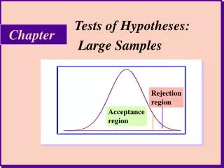
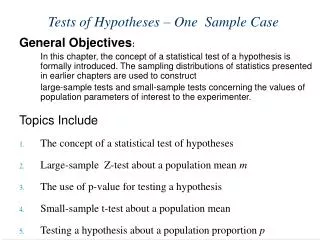
Chapter 9 Large-Sample Tests of Hypotheses General Objectives: In this chapter, the concept of a statistical test of a hypothesis is formally introduced. The sampling distributions of statistics presented in earlier chapters are used to construct large-sample tests concerning the values of population parameters of interest to the experimenter. ©1998 Brooks/Cole Publishing/ITP
Specific Topics 1. A Statistical test of hypotheses 2. Large-sample test about a population mean m 3. Large-sample test about (m1 -m2) 4. Testing a hypothesis about a population proportion p 5. Testing a hypothesis about (p1 -p2) ©1998 Brooks/Cole Publishing/ITP
9.1 Testing Hypotheses About Population Parameters • Samples can be used to estimate the mean potency m of a population. • Two possibilities: - The mean potency m does not exceed the minimum allowable potency. - The mean potency m exceeds the minimum allowable potency. • This is an example of a statistical test of a hypothesis. ©1998 Brooks/Cole Publishing/ITP
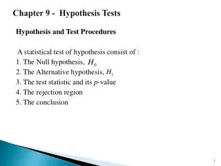
9.2 A Statistical Test of Hypothesis • A statistical test of hypothesis consists of five parts: 1. The null hypothesis, denoted by H0 2. The alternative hypothesis, denoted by Ha 3. The test statistic and its p-value 4. The rejection region 5. The conclusion Definition: The two competing hypotheses are the alternative hypothesisHa, generally the hypothesis that the researcher wishes to support, and the null hypothesisH0, a contradiction of the alternative hypothesis. ©1998 Brooks/Cole Publishing/ITP
The researcher then uses the sample data to decide whether the evidence favors Ha rather than H0 and draws one of these two conclusions: - Reject H0 and conclude that Ha is true. - Accept (do not reject) H0 as true. • Examples 9.1 and 9.2 show null and alternative hypotheses. • You can have a two-tailed test of a hypothesis or a one-tailed test of a hypothesis, a left tailed-test or a right-tailed test. • The test statistic is a single number calculated from sample data. • The p-value is a probability calculated using the test statistic. • Either or both of these measures act as a decision maker for the researcher in deciding whether to reject or accept H0. • Example 9.3 deals with the z-score and the p-value. Figures 9.1 and 9.2 show acceptance and rejection regions. ©1998 Brooks/Cole Publishing/ITP
Example 9.3 For the test of hypothesis in Example 9.1, the average hourly wage for a random sample of 100 California construction workers might provide a good test statistic for testing. If the null hypothesis H0 is true, then the sample mean should not be too far from the population mean m= 14. Suppose that this sample produces a sample mean with standard deviation s= 2. Is this sample evidence likely or unlikely to occur, if in fact H0 is true? You can use two measures to find out. Since the sample size is large, the sampling distribution of is approximately normal with mean m= 14 and standard error The test statistic lies standard deviations from the population mean. ©1998 Brooks/Cole Publishing/ITP
The p-value is the probability of observing a test statistic that is five or more standard deviations from the mean. Since z measures the number of standard deviations a normal random variable lies from its mean, you have The large value of the test statistic and the small p-value mean that you have observed a very unlikely event, if indeed H0 is true and m= 14. ©1998 Brooks/Cole Publishing/ITP
Definition: A Type I error for a statistical test is the error of rejecting the null hypothesis when it is true. The level of significance (significance level)a for a statistical test of a hypothesis is • The value a represents the maximum tolerable risk oF incorrectly rejecting H0. ©1998 Brooks/Cole Publishing/ITP
9.3 A Large-Sample Test About a Population Mean • H0 : m=m0Ha : m>m0 • The standard error of is calculated as • The standardized test statistic: • Figure 9.3 shows a rejection region. Examples 9.4 and 9.5 deal with tests of hypotheses concerning the mean. ©1998 Brooks/Cole Publishing/ITP
Figure 9.3 The rejection region of a right-tailed test with a= .01
Example 9.4 The average weekly earnings for women in managerial and professional positions is $670. Do men in the same positions have average weekly earnings that are higher than those for women? A random sample of n= 40 men in managerial and professional positions showed = $725 and s= $102. Test the appropriate hypothesis using a= .01. Solution You would like to show that the average weekly earnings for men are higher than $670, the women’s average. Hence, if m is the average weekly earnings in managerial and professional positions for men, the hypotheses to be tested are H0 : m= 670versusHa : m> 670 ©1998 Brooks/Cole Publishing/ITP
The rejection region for this one-tailed test consists of large values of or, equivalently, values of the standardized test statistic z in the right tail of the standard normal distribution, with a= .01. This value is found in Table 3 of Appendix I to be z= 2.33, as shown in Figure 9.3. The observed value of the test statistic, using s as an estimate of the population standard deviation, is Since the observed value of the test statistic falls in the rejection region, you can reject H0 and conclude that the average weekly earnings for men in managerial and professional positions are significantly higher than those for women. The probability that you have made an incorrect decision is a= .01. ©1998 Brooks/Cole Publishing/ITP
Figure 9.4 The rejection region for a two-tailed test with a= .01 ©1998 Brooks/Cole Publishing/ITP
The two-tailed hypothesis is written as Ha : m¹m0, which implies either m>m0 or m<m0.. Large-Sample Statistical Test for m: 1. Null hypothesis: H0 : m=m0 2. Alternative hypothesis: One-Tailed Test Two-Tailed Test Ha : m>m0Ha : m¹m0 (or Ha : m<m0) 3. Test statistic: If s is unknown (which is usually the case), substitute the sample standard deviation s for s.. ©1998 Brooks/Cole Publishing/ITP
4. Rejection region: Reject H0 when One-Tailed Test Two-Tailed Test z>zaz>za/2 or z<-za/2 (or z<-za when the alternative hypothesis is Ha : m<m0) • Assumptions: The n observations in the sample are randomly selected from the population and n is large—say, n³ 30. • The unnumbered figures on page 344 show one- and two-tailed rejection regions: ©1998 Brooks/Cole Publishing/ITP
Calculating the p-Value To avoid any ambiguity in their conclusions, some experimenters prefer to use a variable level of significance called the p-value for the test. Definition: The p-value or observed significance level of a statistical test is the smallest value of a for which H0 can be rejected. It is the actual risk of committing a Type I error, if H0 is rejected based on the observed value of the test statistic. The p-value measures the strength of the evidence against H0. • The p-value of the test is actually the area to the right of the calculated value of the test statistic (if the critical value is in the right tail). • Figure 9.5 illustrates variable rejection regions. ©1998 Brooks/Cole Publishing/ITP
Figure 9.5 Variable rejection regions ©1998 Brooks/Cole Publishing/ITP
Definition: If the p-value is less than a preassigned significance level a, then the null hypothesis can be rejected, and you can report that the results are statically significant at level a. • Example 9.6 shows the calculation of thep-value for a two-tailed test. ©1998 Brooks/Cole Publishing/ITP
Example 9.6 Calculate the p-value for the two-tailed test of hypothesis in Example 9.5. Use the p-valueto draw conclusions regarding the statistical test. Solution The rejection region for this two-tailed test of hypothesis is found in both tails of the normal probability distribution. Since the observed value of the test statistic is z=-3.03, the smallest rejection region that you can use and still reject H0 is|z |> 3.03. For this rejection region, the value of a is the p-value: p-value =P(z >3.03)+ P(z <-3.0) =2(.5 - .4988)=2(.0012)=.0024 Notice that the two-tailedp-valueis actually twice the tail area corresponding to the calculated value of the test statistic. If this p-value=.0024 is less than the preassigned level of significance a, H0 can be rejected. For this test, you can reject H0 at either the 1% or the 5% level of significance. ©1998 Brooks/Cole Publishing/ITP
Many researchers use a “sliding scale” to classify their results: - If the p-valueis less than .01, H0 is rejected. The results arehighly significant. - If the p-valueis between .01 and .05, H0 is rejected. The results are statistically significant. - If the p-valueis between .05 and .10, H0 is usually not rejected. The results are only tending toward statistical significance. - If the p-value is greater than .10, H0 is not rejected. The results are not statistically significant. • Example 9.7 conducts a test of hypothesis concerning the mean. ©1998 Brooks/Cole Publishing/ITP
The p-value approach does have two advantages: - Statistical output from packages such as Minitab usually report the p-valueof the test. - Based on the p-value, your test results can be evaluated using any significance level you wish to see. • The smaller the p-value, the more unlikely it is that H0 is true! • Table 9.1 illustrates a decision table. Table 9.1 Null Hypothesis Decision True False Reject H0 Type I error Correct decision Accept H0 Correct decision Type II error ©1998 Brooks/Cole Publishing/ITP
Definition: A Type I error for a statistical test is the error of rejecting the null hypothesis when it is true. The probability of making a Type I error is denoted by the symbol a. A Type II error for a statistical test is the error of accepting (not rejecting) the null hypothesis when it is false and some alternative hypothesis is true. The probability of making a Type II error is denoted by the symbol b. • Notice that the probability of a Type I error is exactly the same as the level of significance aand is therefore controlled by the researcher. • Keep in mind that “accepting” a particular hypothesis means deciding in its favor. • There is always a risk of being wrong, measured by a and b. ©1998 Brooks/Cole Publishing/ITP
Definition: The power of a statistical test, given as 1 - b= P(reject H0 when Ha is true) measures the ability of the test to perform as required. • A graph of (1 - b), the probability ofrejecting H0 when in fact H0 is false, as a function of the true value of the parameter of interest is called the power curve for the statistical test. • Ideally, you would like a to be small and the power (1 - b) tobe large. • Example 9.8 shows the calculation of b and the power of the test (1 - b). ©1998 Brooks/Cole Publishing/ITP
Figure 9.7 Calculating b in Example 9.8 ©1998 Brooks/Cole Publishing/ITP
Figure 9.8 Power curve for Example 9.8 ©1998 Brooks/Cole Publishing/ITP
9.4 A Large-Sample Test of Hypothesis for the Difference Between Two Population Means • In testing whether the difference in sample means indicates that the true difference in populations means differs from a specified value, (m1-m2) = D0, you can use the standard error of the difference in sample means: in the form of a z statistic to measure how many standard deviations the difference lies from the hypothesized difference D0. ©1998 Brooks/Cole Publishing/ITP
Large-Sample Statistical Test for (m1-m2): 1. Null hypothesis: H0 : (m1-m2) =D0, where D0 is some specified difference that you wish to test. For many tests, you will hypothesize that there is no difference between m1 and m2; that is, D0= 0. 2. Alternative hypothesis: One-Tailed Test Two-Tailed Test Ha : (m1-m2) >D0Ha : (m1-m2) ¹D0 [or Ha : (m1-m2) <D0 ] 3. Test statistic: If are unknown (which is usually the case), substitute the sample variances respectively. ©1998 Brooks/Cole Publishing/ITP
4. Rejection region: Reject H0 when One-Tailed Test Two-Tailed Test z>zaz>za/2 or z>-za/2 [or z<-za/2 when the alternative hypothesis is Ha : (m1-m2) <D0 ] or when p-value < m . • Assumptions: The samples are randomly and independently selected from the two populations and n1³ 30 and n2³ 30. ©1998 Brooks/Cole Publishing/ITP
Example 9.9 illustrates a test of the difference in two means. Example 9.9 A university investigation conducted to determine whether car ownership affects academic achievement was based on two random samples of 100 male students, each drawn from the student body. The grade point average for the n1= 100 nonowners of cars had an average and variance equal to as opposed to for the n2= 100 car owners. Do the data present sufficient evidence to indicate a difference in the mean achievements between car owners and nonowners of cars? Test using a = .05. ©1998 Brooks/Cole Publishing/ITP
Solution To detect a difference, if it exists, between the mean academic achievements for nonowners of cars m1 and car owners m2, you will test the null hypothesis that there is no difference between the means against the alternative hypothesis that (m1-m2) ¹ 0;that is, Substituting into the formula for the test statistic, you get ©1998 Brooks/Cole Publishing/ITP
Hypothesis Testing and Confidence Intervals - If the confidence interval you construct contains the value of the parameter specified by H0, then that value is one of the likely or possible values of the parameter and H0 should be rejected. - If the hypothesized value lies outside of the confidence limits, the null hypothesis is rejected at the a level of significance. • Example 9.10 constructs a 95% confidence interval for the difference in average academic achievements. ©1998 Brooks/Cole Publishing/ITP
It is important to understand the difference between results that are “significant” and results that are “practically” important. In statistical language, the word significant does not necessarily mean “ important”, but only that the results could not have occurred by chance. • The unnumbered example on page 364 illustrates a case of statistical versus practical significance. ©1998 Brooks/Cole Publishing/ITP
9.5 A Large-Sample Test of a Hypothesis for a Binomial Proportion Large-Sample Statistical Test for p 1. Null hypothesis: H0 : p = p0 2. Alternative hypothesis: One-Tailed Test Two-Tailed Test Ha : p>p0Ha : p¹p0 (or Ha : p<p0) 3. Test statistic: where x is the number of successes in n binomial trials. ©1998 Brooks/Cole Publishing/ITP
4. Rejection region: Reject H0 when One-Tailed Test Two-Tailed Test z>zaz>za/2 or z>-za/2 (or z<-za/2 when the alternative hypothesis is Ha : p<p0 ) or when p-value <a • Assumption: The sampling satisfies the assumptions of a binomial experiment and n is large enough so that the sampling distribution of can be approximated by a normal distribution(np0 > 5 and nq0 > 5). ©1998 Brooks/Cole Publishing/ITP
Example 9.11 shows a large sample test of hypothesis for a binomial proportion. Example 9.11 Regardless of age, about 20% of American adults participate in fitness activities at least twice a week. However, these fitness activities change as the people get older, and occasional participants become nonparticipants as they age. In a local survey of n= 100 adults over 40 years old, a total of 15 people indicated that they participated in a fitness activity at least twice a week. Do these data indicate that the participation rate for adults over 40 years of age is significantly less than the 20% figure? Calculate the p-valueand use it to draw the appropriate conclusions. Solution It is assumed that the sampling procedure satisfies the requirements of a binomial experiment. You can answer the ©1998 Brooks/Cole Publishing/ITP
question posed by testing the hypothesis A one-tailed test is used because you wish to detect whether the value of p is less than .2. The point estimator of p is and the test statistic is When H0 is true, the value of p is p0= .2, and the sampling distribution of has a mean equal to p0 and a standard deviation of Hence, is not used to estimate the standard error of in this case because the test statistic is calculated under the assumption that H0 is true. (When you estimate the value of p using the estimator , the standard error of is not known and is estimated by ©1998 Brooks/Cole Publishing/ITP
The value of the test statistic is The p-valueassociated with this test is found as the area under the standard normal curve to the left of z= -1.25 as shown in Figure 9.10. Therefore, ©1998 Brooks/Cole Publishing/ITP
9.6 A Large-Sample Test of Hypothesis for the Difference Between Two Binomial Proportions Large-Sample Statistical Test forp1-p2 : 1. Null hypothesis: H0 : (p1-p2) = 0 or equivalently H0 : p1=p2 2. Alternative hypothesis: One-Tailed Test Two-Tailed Test Ha : (p1-p2 ) > 0 Ha : p1-p2 ) ¹ 0 [or Ha : (p1-p2 ) < 0] 3. Test statistic: ©1998 Brooks/Cole Publishing/ITP
where Since the common value of p1=p2=p(used in the standard error) is unknown, it is estimated by and the test statistic is ©1998 Brooks/Cole Publishing/ITP
4. Rejection region: Reject H0 when One-Tailed Test Two-Tailed Test z>zaz>za/2 or z>-za/2 [or z<-za/2 when the alternative hypothesis is Ha : (p1-p2 ) <D0] or when p-value <a • Assumptions: Samples are selected in a random and independent manner from two binomial populations, and n1 and n2 are large enough so that the sampling distribution of can be approximated by a normal distribution. That is, should all be greater than 5. ©1998 Brooks/Cole Publishing/ITP
Example 9.12 illustrates a large-sample statistical test for the difference in two populations and Figure 9.11 shows the location of the rejection region in this example. Figure 9.11 ©1998 Brooks/Cole Publishing/ITP
In some situations, you may need to test for a difference D0 (other than 0) between two binomial proportions. If this is the case, the test statistic is modified for testing H0 : (p1-p2 ) =D0, and a pooled estimate for a common p is no longer used in the standard error. The modified test statistic is Although this test statistic is not used often, the procedure is no different from other large-sample tests you have already mastered! ©1998 Brooks/Cole Publishing/ITP
9.7 Some Comments on Testing Hypotheses • If the p-valueis greater than .05, the results are reported as NS—not significant at the 5% level. • If the p-valuelies between .05 and .01, the results are reported as P < .05—significant at the 5% level. • If the p-valuelies between .01 and .001, the results are reported as P < .01—“highly significant” or significant at the 1% level. • If the p-valueis less that .001, the results are reported as P < .001—“very highly significant” or significant at the .1% level. ©1998 Brooks/Cole Publishing/ITP
Key Concepts and Formulas I. Parts of a Statistical Test 1. Null hypothesis: a contradiction of the alternative hypothesis 2. Alternative hypothesis: the hypothesis the researcher wants to support. 3. Test statistic and its p-value: sample evidence calculated from sample data. 4. Rejection region—critical values and significance levels: values that separate rejection and nonrejection of the null hypothesis 5. Conclusion: Reject or do not reject the null hypothesis, stating the practical significance of your conclusion. ©1998 Brooks/Cole Publishing/ITP
II. Errors and Statistical Significance 1. The significance level a is the probability if rejecting H0 when it is in fact true. 2. The p-valueis the probability of observing a test statistic as extreme as or more than the one observed; also, the smallest value of a for which H0 can be rejected. 3. When the p-valueis less than the significance level a, the null hypothesis is rejected. This happens when the test statistic exceeds the critical value. 4. In a Type II error, b is the probability of accepting H0 when it is in fact false. The power of the test is (1 -b), the probability of rejecting H0 when it is false. ©1998 Brooks/Cole Publishing/ITP
III. Large-Sample Test Statistics Using the z Distribution To test one of the four population parameters when the sample sizes are large, use the following test statistics: ©1998 Brooks/Cole Publishing/ITP