Download
1 / 44
440 likes | 539 Vues
Learn techniques of determining strain or strain rate from displacement or velocity fields in geodesy applications. Understand tensor mathematics, material vs. spatial coordinates, and material derivative for deformation analysis.

E N D
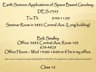
Earth Science Applications of Space Based Geodesy DES-7355 Tu-Th 9:40-11:05 Seminar Room in 3892 Central Ave. (Long building) Bob Smalley Office: 3892 Central Ave, Room 103 678-4929 Office Hours – Wed 14:00-16:00 or if I’m in my office. http://www.ceri.memphis.edu/people/smalley/ESCI7355/ESCI_7355_Applications_of_Space_Based_Geodesy.html Class 12
Determining Strain or strain rate from Displacement or velocity field Deformation tensor Strain (symmetric) and Rotation (anti-symmetris) tensors
Write it out Deformation tensor is not symmetric, have to keep dxy and dyx. Again – this is “wrong way around” We know u and x and want t and dij.
So rearrange it Now we have 6 unknowns and 2 equations
So we need at least 3 data points That will give us 6 data And again – the more the merrier – do least squares.
For strain rate Take time derivative of all terms. But be careful Strain rate tensor is NOT time derivative of strain tensor.
Spatial (Eulerian) and Material (Lagrangian) Coordinates and the Material Derivative Spatial description picks out a particular location in space, x. Material description picks out a particular piece of continuum material, X.
So we can write x is the position now (at time t) of the section that was initially (at time zero) located at A. or A was the initial position of the particle now at x This gives by definition
We can therefore write Next consider the derivative (use chain rule)
Define Material Derivative Vector version
Example Consider bar steadily moving through a roller that thins the bar A Examine velocity as a function of time of cross section A
The velocity will be constant until the material in A reaches the roller At which point it will speed up (and get a little fatter/wider, but ignore that as second order) After passing through the roller, its velocity will again be constant A(t=t1) A(t=t2)
v(x1) v(x2) If one looks at a particular position, x, however the velocity is constant in time. So for any fixed point in space A(t=t1) A(t=t2) So the acceleration seems to be zero (which we know it is not)
v(x1) v(x2) The problem is that we need to compute the time rate of change of the material which is moving through space and deforming (not rigid body) (we want/need our reference frame to be with respect to the material, not the coordinate system. A(t=t1) A(t=t2)
v(x1) v(x2) We know acceleration of material is not zero. A(t=t1) A(t=t2) Term gives acceleration as one follows the material through space (have to consider same material at t1 and t2)
Various names for this derivative Substantive derivative Lagrangian derivative Material derivative Advective derivative Total derivative
GPS and deformation Now we examine relative movement between sites
Strain-rate sensitivity thresholds (schematic) as functions of period GPS and INSAR detection thresholds for 10-km baselines, assuming 2-mm and 2-cm displacement resolution for GPS and INSAR, respectively (horizontal only). http://www.iris.iris.edu/USArray/EllenMaterial/assets/es_proj_plan_lo.pdf, http://www.iris.edu/news/IRISnewsletter/EE.Fall98.web/plate.html
Strain-rate sensitivity thresholds (schematic) as functions of period Post-seismic deformation (triangles), slow earthquakes (squares), long-term aseismic deformation (diamonds), preseismic transients (circles), and volcanic strain transients (stars). http://www.iris.iris.edu/USArray/EllenMaterial/assets/es_proj_plan_lo.pdf, http://www.iris.edu/news/IRISnewsletter/EE.Fall98.web/plate.html
Study deformation at two levels • ------------- • Kinematics – • describe motions • (Have to do this first) • ---------------- • Dynamics – • relate motions (kinematics) to forces (physics) • (Do through rheology/constitutive relationship/model. • Phenomenological, no first principle prediction)
Simple rheological models elastic e(s) e s http://hcgl.eng.ohio-state.edu/~ce552/3rdMat06_handout.pdf
Simple rheological models viscous e2 (t) s e s2 e1 (t) s1 t t ta tb Apply constant stress, s, to a viscoelastic material. Record deformation (strain, e) as a function of time. e increases with time. http://hcgl.eng.ohio-state.edu/~ce552/3rdMat06_handout.pdf
Simple rheological models viscous e s e2 s2 (t) e1 s1 (t) t t tb ta Maintain constant strain, record load stress needed. Decreases with time. Called relaxation. http://hcgl.eng.ohio-state.edu/~ce552/3rdMat06_handout.pdf
viscoelastic Kelvin rheology Handles creep and recovery fairly well Does not account for relaxation http://hcgl.eng.ohio-state.edu/~ce552/3rdMat06_handout.pdf
viscoelastic Maxwell rheology Handles creep badly (unbounded) Handles recovery badly (elastic only, instantaneous) Accounts for relaxation fairly well http://hcgl.eng.ohio-state.edu/~ce552/3rdMat06_handout.pdf
viscoelastic Standard linear/Zener (not unique) Spring in parallel with Maxwell Spring in series with Kelvin Stress – equal among components in series Total strain – sum all components in series Strain – equal among components in parallel Total stress – total of all components in parallel http://hcgl.eng.ohio-state.edu/~ce552/3rdMat06_handout.pdf www.mse.mtu.edu/~wangh/my4600/chapter4.ppt
viscoelastic Standard linear/Zener Instantaneous elastic strain when stress applied Strain creeps towards limit under constant stress Stress relaxes towards limit under constant strain Instantaneous elastic recovery when strain removed Followed by gradual recovery to zero strain http://hcgl.eng.ohio-state.edu/~ce552/3rdMat06_handout.pdf www.mse.mtu.edu/~wangh/my4600/chapter4.ppt
viscoelastic Standard linear/Zener Two time constants - Creep/recovery under constant stress - Relaxation under constant strain http://hcgl.eng.ohio-state.edu/~ce552/3rdMat06_handout.pdf www.mse.mtu.edu/~wangh/my4600/chapter4.ppt
Can make arbitrarily complicated to match many deformation/strain/time relationships http://www.dow.com/styron/design/guide/modeling.htm
Three types faults and plate boundaries ----------------------- - Faults - Strike-slip Thrust Normal --------------------------- - Plate Boundary - Strike-slip Convergent Divergent
How to model ------------------- Elastic Viscoelastic ---------------------- Half space Layers Inhomogeneous
2-D model for strain across strike-slip fault in elastic half space. Fault is locked from surface to depth D, then free to infinity. Far-field displacement, V, applied.
w(x) is the equilibrium displacement parallel to y at position x. |w| is 50% max at x/D=.93; 63% at x/D=1.47 & 90% at x/D=6.3
Effect of fault dip. The fault is locked from the surface to a depth D (not a down dip length of D). The fault is free from this depth to infinity.
Surface deformation pattern is SAME as for vertical fault, but centered over down dip end of dipping fault. Dip estimation from center of deformation pattern to surface trace and locking depth.
Interseismic velocities in southern California from GPS Meade and Hager, 2005
Fault parallel velocities for northern and southern “swaths”. Total change in velocity ~42mm/yr on both. Meade and Hager, 2005
Residual (observed-model) velocities for block fault model (faults in grey) Meade and Hager, 2005
Modeling velocities in California • is the angular velocity vector effect of interseismic strain accumulation is given by an elastic Green's function G response to backslip distribution, s, on each of, f, faults. Modeling Broadscale Deformation From Plate Motions and Elastic Strain Accumulation, Murray and Segall, USGS NEHRP report.
In general, the model can accommodate zones of distributed horizontal deformation if W varies within the zones latter terms can account both for the Earth's sphericity and viscoelastic response of the lower crust and upper mantle. Modeling Broadscale Deformation From Plate Motions and Elastic Strain Accumulation, Murray and Segall, USGS NEHRP report.
Where a is the Earth radius distance from each fault located at ff is a(f-ff). Each fault has deep-slip rate aDwfsinff, where Dwf is the difference in angular velocity rates on either side of the fault. Modeling Broadscale Deformation From Plate Motions and Elastic Strain Accumulation, Murray and Segall, USGS NEHRP report.