Comprehensive Genetic Model Framework for Population Parameters and Allelic Transmission
This document outlines a robust framework for understanding genetic models by detailing population parameters, transmission dynamics, and penetrance relationships. It discusses key components like alleles, genotypes, mating types, and their influence on offspring inheritance through Mendelian laws. Additionally, it explores the statistical implications of identity by descent (IBD) and identity by state (IBS) in sibling pairs, alongside the estimation of genetic correlations and the effects of recombination on genotype distributions. This comprehensive approach aims to enhance our understanding of quantitative traits and their genetic basis.

Comprehensive Genetic Model Framework for Population Parameters and Allelic Transmission
E N D
Presentation Transcript
Genetic Theory Pak Sham SGDP, IoP, London, UK
Inference Interpretation Formulation Experiment Data Theory Model
Components of a genetic model • POPULATION PARAMETERS • - alleles / haplotypes / genotypes / mating types • TRANSMISSION PARAMETERS • - parental genotype offspring genotype • PENETRANCE PARAMETERS • - genotype phenotype
½ ½ ½ A A A A ¼ ¼ A A A A ¼ ¼ ½ Transmission : Mendel’s law of segregation Maternal A A A Paternal A
AAAA AA AA AAAA AA AA AAAA AA AA AAAA AA AA AAAA AA AA AAAA AA AA AAAA AA AA AAAA AA AA Two offspring Sib 2 AA AAAA AA AA AA AA AA S i b 1
IBD sharing for two sibs AA AAAA AA 0 AA AA AA AA 2 1 1 1 1 2 0 1 1 0 2 2 0 1 1 Expected IBD sharing = (2*0.25) + (1*0.5) + (0*0.25) = 1 Pr(IBD=0) = 4 / 16 = 0.25 Pr(IBD=1) = 8 / 16 = 0.50 Pr(IBD=2) = 4 / 16 = 0.25
IBS IBD A1A2 A1A3 IBS = 1 IBD = 0 A1A2 A1A3
Y X - expected IBD proportion = (½)5 +(½)5 = 0.0625 1 via X : 5 meioses via Y : 5 meioses 2 - identify all nearest common ancestors (NCA) - trace through each NCA and count # of meioses
Sib pairs Expected IBD proportion = 2 (½)2 = ½
Likely (1-) = recombination fraction Unlikely () Segregation of two linked loci Parental genotypes
Recombination & map distance Haldane map function
(1-1)(1-2) (1-1)2 1(1-2) 12 Segregation of three linked loci 1 2
Two-locus IBD distribution: sib pairs • Two loci, A and B, recombination faction • For each parent: • Prob(IBD A = IBD B) = 2 + (1-)2 = • either recombination for both sibs, • or no reombination for both sibs
Conditional distribution of at maker given at QTL at QTL 0 1/2 1 at M 0 1/2 1
Correlation between IBD of two loci • For sib pairs • Corr(A, B) = (1-2AB)2 • attenuation of linkage information with increasing genetic distance from QTL
Population Frequencies • Single locus • Allele frequencies A P(A) = p • a P(a) = q • Genotype frequencies • AA p(AA) = u • Aa p(Aa) = v • aa p(aa) = r
Mating type frequencies • uv r • AA Aa aa • u AA u2 uvur • v Aa uvv2 vr • r aa urvrr2 • Random mating
Hardy-Weinberg Equilibrium • u+½v r+½v • A a • u+½v A • r+½v a u1 = (u0 + ½v0)2 v1 = 2(u0 + ½v0) (r0 + ½v0) r1 = (r0 + ½v0)2 u2 = (u1 + ½v1)2 = ((u0 + ½v0)2 + ½2(u0 + ½v0) (r0 + ½v0))2 = ((u0 + ½v0)(u0 + ½v0 + r0 + ½v0))2 = (u0 + ½v0)2 = u1
Hardy-Weinberg frequencies • Genotype frequencies: • AA p(AA) = p2 • Aa p(Aa) = 2pq • aa p(aa) = q2
Two-locus: haplotype frequencies • Locus B • B b • Locus A A AB Ab • a aB ab
Haplotype frequency table • Locus B • B b • Locus A A pr ps p • a qr qs q • r s
Haplotype frequency table • Locus B • B b • Locus A A pr+D ps-D p • a qr-D qs+D q • r s • Dmax = Min(ps,qr), D’ = D / Dmax • R2 = D2 / pqrs
Causes of allelic association • Tight Linkage • Founder effect: D (1-)G • Genetic Drift: R2 (NE)-1 • Population admixture • Selection
Genotype-Phenotype Relationship • Penetrance = Prob of disease given genotype • AA Aa aa • Dominant 1 1 0 • Recessive 1 0 0 • General f2 f1 f0
Biometrical model of QTL effects • Genotypic • means • AA m + a • Aa m + d • aa m - a 0 -a +a d
Quantitative Traits • Mendel’s laws of inheritance apply to complex traits • influenced by many genes • Assume: 2 alleles per locus acting additively • Genotypes A1 A1 A1 A2 A2 A2 • Effect -1 0 1 • Multiple loci • Normal distribution of continuous variation
1 Gene 3 Genotypes 3 Phenotypes 2 Genes 9 Genotypes 5 Phenotypes 3 Genes 27 Genotypes 7 Phenotypes 4 Genes 81 Genotypes 9 Phenotypes Quantitative Traits
Components of variance • Phenotypic Variance • Environmental Genetic GxE interaction
Components of variance • Phenotypic Variance • Environmental Genetic GxE interaction • Additive Dominance Epistasis
Components of variance • Phenotypic Variance • Environmental Genetic GxE interaction • Additive Dominance Epistasis • Quantitative trait loci
Biometrical model for QTL • Genotype AA Aa aa • Frequency (1-p)2 2p(1-p) p2 • Trait mean -a d a • Trait variance 2 2 2 • Overall mean a(2p-1)+2dp(1-p)
QTL Variance Components • Additive QTL variance • VA = 2p(1-p) [ a - d(2p-1) ]2 • Dominance QTL variance • VD = 4p2 (1-p)2 d2 • Total QTL variance • VQ = VA + VD
Covariance between relatives • Partition of variance Partition of covariance • Overall covariance • = sum of covariances of all components • Covariance of component between relatives • = correlation of component • variance due to component
Correlation in QTL effects • Since is the proportion of shared alleles, correlation in QTL effects depends on • 0 1/2 1 • Additive component 0 1/2 1 • Dominance component 0 0 1
Average correlation in QTL effects • MZ twins P(=0) = 0 • P(=1/2) = 0 • P(=1) = 1 • Average correlation • Additive component = 0*0 + 0*1/2 + 1*1 • = 1 • Dominance component = 0*0 + 0*0 + 1*1 • = 1
Average correlation in QTL effects • Sib pairs P(=0) = 1/4 • P(=1/2) = 1/2 • P(=1) = 1/4 • Average correlation • Additive component = (1/4)*0+(1/2)*1/2+(1/4)*1 • = 1/2 • Dominance component = (1/4)*0+(1/2)*0+(1/4)*1 • = 1/4
Decomposing variance E Covariance A C 0 Adoptive Siblings 0.5 1 DZ MZ
Path analysis • allows us to diagrammatically represent linear models for the relationships between variables • easy to derive expectations for the variances and covariances of variables in terms of the parameters of the proposed linear model • permits translation into matrix formulation (Mx)
Variance components Dominance Genetic Effects Additive Genetic Effects Shared Environment Unique Environment E C A D e c a d Phenotype P = eE + aA + cC + dD
ACE Model for twin data 1 [0.5/1] E C A A C E e c a a c e PT1 PT2
QTL linkage model for sib-pair data 1 [0 / 0.5 / 1] N S Q Q S N n s q q s n PT1 PT2
Inference Interpretation Formulation Experiment Data Theory Model