Download
1 / 14
140 likes | 222 Vues
This study explores a novel approach for setting due dates in complex product systems with uncertain processing times. It introduces a methodology involving leadtime distribution estimation, due date planning strategies, and an industrial case study analysis. The research aims to enhance delivery performance, address uncertainties, and improve assembly processes in such systems. The approximate procedure developed in this work offers a practical solution for due date determination in scenarios with stochastic processing times. The findings of the study provide valuable insights for efficient planning in complex manufacturing environments.

E N D
Due Date Planning for Complex Product Systemswith Uncertain Processing Times By: D.P. Song,C.Hicks and C.F.Earl Dept. of MMM Eng. Univ. of Newcastle upon Tyne 2nd Int. Conf. on the Control of Ind. Process, March, 30-31, 1999
Overview 1. Introduction 2. Literature Review 3. Simple Two Stage System 4. Leadtime Distribution Estimation 5. Due Date Planning 6. Industrial Case Study 7. Discussion and Further Work
Introduction • Delivery performance • Uncertainties • Complex product system • Assembly • Product structure • Problem : setting due date in complex product systems withuncertainprocessing times
Literature Review Two principal research streams [Cheng(1989), Lawrence(1995), Philipoom(1997)] • Empirical method: based on job characteristics and shop status. Such as: TWK, SLK, NOP, JIQ, JIS • Analytic method: queuing networks, mathematical programming etc.by minimising a cost function Limitation of above research • Both focus on job shop situations • Empirical -- time consuming in stochastic systems • Analytic -- limited to “small” problems
Our approximate procedure • Using analytical/numerical method Þ moments of two stage leadtime Þ approximate distribution Þ decompose into two stages Þ approximate total leadtime Þ set due date
Simple Two Stage System • Product structure Fig. 1 A two stage assembly system
Analytical Result • Cumul. Distr. Func.(CDF) of leadtime W is: FW(t)= 0, t<M1+S1; FW(t) = F1(M1) FZ(t-M1) + F1¢ÄFZ, t ³ M1 + S1. where M1 ¾ minimum assembly time S1 ¾ planned assembly start time F1 ¾ CDF of assembly processing time; FZ¾ CDF of actual assembly start time; FZ(t)= P1n F1i(t-S1i) ľ convolution operator in [M1, t - S1]; F1¢ÄFZ= òF1¢(x) FZ(x-t)dx
Leadtime Distribution Estimation Assumptions • normally distributed processing times • approximate leadtime by normal distr.(Soroush,1999) Approximating leadtime distribution • Compute mean and variance of assembly start time Z and assembly process time Q : mZ, sZ2andmQ, sQ2 • Obtain mean and variance of leadtime W(=Z+Q): mW = mQ+mZ, sW2 = sQ2+sZ2 • Approximate W by normal distribution: N(mW, sW2), t ³ M1+ S1.
Due Date Planning • Mean absolute lateness Þd* = median • Standard deviation lateness Þd* = mean • Asymmetric earliness and tardiness cost Þd* by root finding method • Achieve a service target Þd* by N(0, 1)
Industrial Case Study • Product structure 17 components 17 components Fig. 2 An practical product structure
System parameters setting • normal processing times • at stage 6: m =7days for 32 components, m =3.5 days for the other two. • at other stages : m=28 days • standard deviation: s= 0.1m • backward scheduling based on mean data • planned start time: 0 for 32 components and 3.5 for other two.
Leadtime distribution comparison Fig. 3 Approximation PDF and Simulation histogram of total leadtime
Due date results comparison Table. Due dates to achieve service targets by simulation and approximation methods
Discussion & Further Work • Production plan/Minimum processing times • Skewed distributed processing times • More general distribution to approximate, like l-type distribution • Resource constraint systems