Analysis of the entrainment on lock-exchange gravity currents

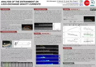
1. Analysis of the entrainment on lock-exchange gravity currents H.I.S. Nogueira1, C. Adduce2, E. Alves3, M.J. Franca1,4 1University of Coimbra & IMAR-CMA, Coimbra, Portugal (hnogueira@dec.uc.pt) 2 University of Rome “Roma Tre”, Rome, Italy 3 National Laboratory of Civil Engineering, Lisbon, Portugal 4 New University of Lisbon & IMAR-CMA, Caparica, Portugal 1. Introduction 3. Calibration method 4. Results Entrainment rate The evaluation of the current density distribution was based on Hacker et al. (1996) technique, which relates light intensity through the current with concentration of dye present in the flow; this later is considered linearly correlated with salt concentration within the current body. A calibration procedure was carried out for each run and for each single pixel to establish the relation between the amount of dye in the water and the values of gray scale in the frames representing light intensities. Assuming a direct relation between the amount of dye and the density of the current, it is thus possible to infer density values at any given pixel and at any given instant from its instantaneous gray scale value. The estimation of pixel density is made by means of a cubic interpolation applied to the local calibration curve (Fig. 2). The mass conservation equation (MCE) is presented below in the integral form for a moving and deforming control volume defining the current head. As our main goal is to estimate the entrainment rate of ambient fluid into the current head, the convective term, representing the fluxes through the boundaries in the MCE, was divided in two, representing mass fluxes through the internal and external boundaries, respectively. local convective csint csext external boundary internal boundary cv Fig.4 shows the main results regarding the head dynamics, where length and time are normalized as following , , being the buoyancy velocity. The aim of the present work is to experimentally investigate the entrainment rate of ambient fluid into the region of current head of unsteady density currents performed by lock-exchange releases of saline water into a fresh water tank. a) d) . 1 . 5 . 6 . 2 Fig. 2 Example of images used for calibration and corresponding calibration curve obtained for one central pixel of the image represented in the frames by a white dot. 2. Experimental procedure b) e) . 3 . 7 The experiments were carried out at the Hydraulics Laboratory of University “Roma Tre”, in a 3.0 m long transparent Perspex channel with a 0.2 m wide and 0.3 m deep rectangular cross-section (Fig.1). A vertical sliding gate is placed in the channel at a distance x0 from the left wall to form a lock. The right side of the channel is filled with fresh water with density ρ0, whereas the lock is filled with saline water with density ρ1, both sides filled up at same depth, h0. A controlled quantity of dye is added to the water in the lock to provide flow visualization. Fig. 1 Perspex channel. a) perspective view and b) longitudinal view. When the gate is suddenly removed, a gravity current is established by the dense fluid flowing under the fresh water. The evolution of the gravity current is recorded by a CCD video camera with a frequency of 25 Hz kept at a fixed position 5.8 m from the channel. The illumination was made by means of artificial light. The instantaneous density field of the current was assessed through an image analysis technique applied to the video frames. These, with 768 x 576 pixel points, were subsequently converted into gray scale matrices and then converted into instantaneous density fields of the current through a nonlinearcalibration method. Eight different lock-exchange tests were preformed varying the initial density of the saline water, the water depth and bed roughness. Herein we present the results for only one experiment (run D1 in the table below). Table 1 Description of the lock-exchange experiments 4. Results 2D Density fields Fig. 3 shows the development of the current captured in three instants and the corresponding normalized instantaneous density fields . Kelvin-Helmholtz type instabilities are quite visible at the mixing layer of the current and exhibit a quasi stationary behaviour. Since the head of the current is a region of higher density, the criteria used to characterize and isolate this region was based on the product between the local density, vertically averaged, and current height: .The upstream limit of the head, and therefore the head lengthLf, were defined taking the position of the local minimum of the function near the front. • experimental data • linear regression . 4 . 8 c) f) Density or gravity currents are geophysical flows driven by density differences within a fluid, which can be caused by temperature differences, dissolved substances or particles in suspension. Oceanic fronts and turbidity currents in lakes and reservoirs are examples of gravity currents occurring in masses of water. The latter may occur as a result of human intervention (release of mineral waste, dredging operations) or spontaneously in nature (flood events, earthquakes) in natural lakes and in the deep ocean, with significant morphological impacts. The understanding of the mechanisms involving these large-scale phenomena is thus of extreme importance for the development of prevention measures against their eventual adverse effects. In the total mass conservation equation, the entrainment rate of the ambient fluid through the upper interface becomes a source term requiring a closure model. The entrainment rate may be modeled as a function of the buoyancy velocity and a characteristic density, and it is usually evaluated through empirical relations. a) b) Gate KH Billow Fig. 4 a) Front position, b) front velocity, c) head length, d) mass of the head, e) local and convective terms of MCE and f) entrainment coefficient. Lock 0.3 m t = 19.6 s ρ1 ρ0 h0 t * = 16.8 z x 0 5. Discussion Lf x0 The front velocity (Fig.4b) was obtained from the front position xf(t) by its derivative in time using centred finite differences of 2nd order. Front velocity decays linearly, besides the oscillations, which is in accordance with the shape of the x*fplot (Fig. 4a). As the current advances, the front motion is characterized by repeated cycles of stretching+break(Fig. 4c and 4d), where mass detachment from the head towards upstream, into the current body, is observed. This cyclic behaviour (with period of roughly T* = 1.8) influences consequently the MCE terms (Fig. 4e) and in the entrainment coefficient (Fig. 4f). Since the internal boundary flux term is positive, conservation of mass implies that the remaining flux through the external boundary to be negative (inwards), corresponding to entrainment of water into the current head. Fig. 4f) shows a decreasing entrainment rate in time, as expected, converging asymptotically to a plateau at Ea = 0. 3.0 m t = 27.6 s t * = 23.7 t = 35.6 s t * = 30.6 Financial support This research was supported by the Portuguese Science and Technology Foundation through the research project PTDC/ECM/099752/2008 and the research grant SFRH/BD/48705/2008. Fig. 3 Photos of the current acquired in run D1 and corresponding density fields.