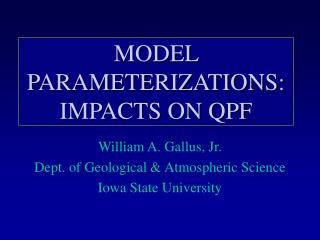
MODEL PARAMETERIZATIONS: IMPACTS ON QPF
MODEL PARAMETERIZATIONS: IMPACTS ON QPF. William A. Gallus, Jr. Dept. of Geological & Atmospheric Science Iowa State University. GOOD NEWS: QPF is improving!!. Increased computer resources have allowed better parameterization schemes and model resolution

MODEL PARAMETERIZATIONS: IMPACTS ON QPF
E N D
Presentation Transcript
MODEL PARAMETERIZATIONS:IMPACTS ON QPF William A. Gallus, Jr. Dept. of Geological & Atmospheric Science Iowa State University
GOOD NEWS: QPF is improving!! Increased computer resources have allowed better parameterization schemes and model resolution 2-day precipitation forecast today is now as accurate as 1-day forecast in 1974 Each resolution improvement in NCEP Eta model improves skill scores
BAD NEWS: Problems abound Most improvement in QPF scores occurs during cold season - little improvement in warm season Flash flooding kills more people than any other convective-related event QPF problems have several potential sources Skill scores used to evaluate forecasts themselves may be misleading or of little “real” value
Slow improvement in skill for human forecasters, but less skill for heavier amounts (Olson et al. 1995, WAF)
What are sources of QPF error? • Resolution • Initialization • Parameterization How do these interact?
What is the impact of resolution? • For convection: not straightforward -- depends on parameterizations • For stable precipitation: depends on parameterizations also
Gallus 1999 found QPF-horizontal resolution dependence is case-dependent and varies with convective parameterization 6/16/96 6/14/98 7/28/97 Mx obs: 225 Mx obs: 330 Mx obs: 250 5/27/97 7/17/96 Mx obs: 102 Mx obs: 300 BMJ -shaded KF - clear
Extreme example of unexpected results and Conv. Param. Impacts: 7/17/96 00UTC surface conditions
00 UTC 17 JUL 1996 - OMAHA Betts-Miller-JanjicReference T, Td profiles shown
Large MCS drops up to 300 mm of rain, causing record river crests and severe flash flooding in far eastern NE and western IA.
7/17/96 BMJ simulations with 78,39,22 and 12 km horizontal resolution NOTE: actual reduction in peak QPF amounts as resolution improves MX: 46 MX: 45 MX: 32 MX: 32
7/17/96 KF simulations: NOTE: very strong QPF sensitivity to horizontal resolution. Precipitation area shifted much farther north than in BMJ runs, or observations MX: 70 MX: 11 MX: 135 MX: 186
Daytime precipitation (12-00 UTC 7/16-17/96) BMJ produces much larger area and amounts
KF BMJ Convective scheme influences cold pool strength, which in turn, affects evolution of events outside initial rain region
Impacts of convective schemes may be felt outside region of precipitation. Here, stronger downdrafts in KF scheme result in greater northward transport of instability into Minnesota - leading to more intense subsequent development. KF BMJ
Another case: Iowa flood of June 1996 Large-scale region looked favorable for excessive rains Heaviest rains (225 mm) fell in small area in warm sector Impacts of horizontal resolution changes strongly depend on convective scheme used
Tropical-like soundings with very deep moisture Td at 850 mb = 18 C Td at 700 mb = 8 C
BMJ simulations: Almost no horizontal resolution-QPF dependence No hint of C IA maximum
21 UTC 6/16 Observed Surface Moisture Convergence Flood-producing storms would form on C IA enhancement
Simulated Moisture Convergence -21 UTC - BMJ run with 12 km resolution Despite poor initial wind field, model does show enhancement in W IA
BMJ simulation: No general clearing into Iowa by 1 pm - Less destabilization than actually occurred
KF simulations: Strong horizontal resolution-QPF dependence Some evidence of C IA enhancement with 22 and 12 km resolution
KF 6 hr forecast: Some clearing into SW Iowa more agreement with obs.
June case shows: • Moist low-mid troposphere allows BMJ scheme to be aggressive • Even high resolution may not improve simulation of small QPF maxima if other simulated parameters are incorrect • Generation of QPF upstream due to resolution changes may affect QPF downstream
For non-convective precipitation, sensitivities to grid spacing and microphysical parameterization can be significant • Colle and Mass examine resolution-orographic precipitation (1999) dependence • Microphysical schemes influence results
OBS PRECIP IN PACIFIC NORTHWEST FLOOD EVENT (1996) from Colle and Mass (1999; MWR) Pronounced orographic effects
4 km MM5 run does well at crest but underestimates lee precipitation
Horizontal resolution affects precipitation patterns near mountain due to resolution of mountain wave effects. Model QPF performance in lee of mountain fluctuates - low bias is best in coarsest run, but heaviest precipitation just to lee of crest occurs with highest resolution 1.33 4 12 36
Microphysical schemes may have significant influences at high resolution. Colle and Mass (1999; MWR) found that lee-side precipitation was too small in high-res MM5 simulations, partly because snow fallspeeds were too large.
Best results may not occur with most sophisticated microphysical scheme
Microphysical scheme differences affect QPF in different areas
What impact does initialization have? • Although impacts can be significant in some cases, recent ensemble work suggests parameterization details have bigger impact on short-term mesoscale forecasts
10 km Eta simulations run for 20 cases of Midwest MCSs • Improvements in initialization to better depict mesoscale features generally result in limited improvement in skill scores • Variations in forecast are much larger for change in convective parameterization than for any change in initial conditions
.01 .05 .10 .15 .20 .25 .35 .50 1.0 BMJ MO CP KF ETS Scores averaged over 50 periods
What impact does initialization have? • Although impacts can be significant in some cases, recent ensemble work suggests parameterization details have bigger impact on short-term mesoscale forecasts • One example in one case: Gallus and Segal (2000) found potentially strong sensitivity of QPF to soil moisture, but depended greatly on choice of convective scheme
Impact of varied soil moisture on QPF depends greatly on convective scheme. With BMJ - wetter soil yields heavier peak QPF With KF - heaviest QPF occurs with dry soil due to stronger low-level winds and previous outflow
Parameterizations are clearly a primary influence on QPF:Which are key? • Convective Parameterizations • Land-Surface/Boundary Layer Schemes • Microphysical parameterizations (also influence radiative schemes)
Ways for Convective Schemes to activate: • Presence of instability at grid point • Existence of low or mid-level mass or moisture convergence exceeding threshold • Rate of destabilization at a grid point
How does convection affect the larger-scale? • Adjustment schemes nudge toward empirical curves, a function of difference between the moist adiabats of cloud and environment • Mass flux schemes explicitly model convective feedback at each grid point
Let’s examine primary NCEP models • ETA: 22 km horizontal resolution/50 layers - uses BMJ (adjustment w/o downdraft) test version uses KF (mass flux w downdraft) • RUC: 20 km horizontal resolution/40 layers - uses Grell (mass flux w downdraft) • AVN: 70 km horizontal resolution/42 layers - uses Grell-Pan (mass flux) for deep with Tiedke (mass flux w downdraft) for shallow
Operational Eta: • In BMJ scheme, both shallow and deep convection occur. • Deep convection potential is first evaluated • Shallow convection only occurs if no deep convection is present
Deep Convection • Most unstable parcel in lowest 200* hPa • Cloud depth must exceed 200 hPa (or less if terrain is elevated) • Reference Temp profile in cloud layer has 90% of slope of moist adiabat at cloud base • Reference Moisture profile based on deficit from saturation pressure at cloud base, freezing level and cloud top
Deep Convection (cont.) • Modification made for precipitation efficiency (less mature system has larger P.E.) • PE is a measure of how well the cloud transports enthalpy upward vs. how much precip is produced • If negative precipitation is produced by convective adjustment toward moisture profile, shallow scheme is called
00 UTC 17 JUL 1996 - OMAHA Betts-Miller-JanjicReference T, Td profiles shown
Shallow BMJ scheme • Clouds must be 10-200 hPa deep • Lower cloud is warmed/dried while upper portion is cooled and moistened • Moist mixing process can help the deep convection to later activate, but also result in unrealistic thermodynamic profiles
Effect of Eta BMJ shallow convection - from Baldwin et al. 2000
Eta: KF Scheme • Activated by more traditional trigger function - W • Mass flux scheme with parameterized downdrafts • Original scheme much less aggressive than BMJ - more grid-resolved precipitation, but changes have made it more like BMJ (though still with lower bias scores)
Any general rules about the Eta convective schemes? • BMJ generally likes moist environments - usually rain areas are too broad and not intense enough • KF may be better in showing heavier amounts in small regions, and in activating along dry lines • BMJ traditionally was too dry in elevated terrain of West USA (change in cloud depth may improve this dry bias)