Channel Assignment in Cellular Networks

1. Channel Assignment in Cellular Networks Ivan Stojmenovic www.site.uottawa.ca/~ivan Ivan@site.uottawa.ca

2. Overview • Fixed channel assignment • Multicoloring – co-channel interference • General problem statement • Genetic algorithms • Results and details • Fixed/dynamic channel and power assignment

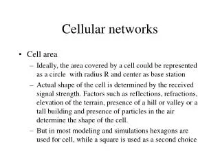
3. Cell structure • Implements space division multiplex: base station covers a certain transmission area (cell) • Mobile users communicate only via the base station • Advantages of cell structures: • higher capacity, higher number of users • less transmission power needed • more robust, decentralized • base station deals with interference locally • Cell sizes from some 100 m in cities to, e.g., 35 km on the country side (GSM) - even more for higher frequencies

4. Cellular architecture One low power transmitter per cell Frequency reuse–limited spectrum Cell splitting to increase capacity B A Reuse distance:minimum distance between two cells using same channel for satisfactory signal to noise ratio Measured in # of cells in between

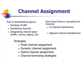
5. Problems • Propagation path loss for signal power: quadratic or higher in distance • fixed network needed for the base stations • handover (changing from one cell to another) necessary • interference with other cells: • Co-channel interference: Transmission on same frequency • Adjacent channel interference: Transmission on close frequencies

6. Reuse pattern for reuse distance 2? One frequency can be (re)used in all cells of the same color Minimize number of frequencies=colors

7. Reuse distance 2 – reuse pattern One frequency can be (re)used in all cells of the same color

8. Reuse pattern for reuse distance 3?

9. Reuse distance 3 – reuse pattern

10. Frequency planning I f3 f5 f2 f4 f6 f5 f1 f4 f3 f7 f1 f2 • Frequency reuse only with a certain distance between the base stations • Standard model using 7 frequencies: • Note pattern for repeating the same color: one north, two east-north

11. Fixed and Dynamic assignment • Fixed frequency assignment: permanent • certain frequencies are assigned to a certain cell • problem: different traffic load in different cells • Dynamic frequency assignment: temporary • base station chooses frequencies depending on the frequencies already used in neighbor cells • more capacity in cells with more traffic • assignment can also be based on interference measurements

12. 3 cell clusterwith 3 sector antennas f2 f2 f2 f1 f1 f1 h2 f3 h2 f3 f3 h1 h1 h3 h3 g2 g2 g2 g1 g1 g1 g3 g3 g3

13. Cell breathing • CDM systems: cell size depends on current load • Additional traffic appears as noise to other users • If the noise level is too high users drop out of cells

14. Multicoloring • Weight w(v) of cell v = # of requested frequencies • Reuse distance r • Minimize # channels used: NP hard problem • Multi-coloring = multi-frequencing • Channel= Frequency= Color • Hybrid CA = combination fixed/dyn. frequencies • Graph representation: weighted nodes, two nodes connected by edge iff their distance is < r • same colors cannot be assigned to edge endpoints

15. Hexagon graphs: reuse distance 2 What is the graph for reuse distance 3?

16. Lower bounds for hexagonal graphs D= Maximum total weight on any clique Lower bound on number of channels: D D/3 D/2 D/2 Needs 9/8D channels D/2 D/2 0 D/2 D/6 0 0 D/2 D/2 D/2 D/2 D/2 Odd cycle bound: induced 9-cycle, each weight D/2 Channels needed in this cycle: 9D/2 Each channels can be used at most 4 times.

17. Fixed allocations – reuse distance 2 D= maximum number of channels in a node or 3-cycle Red : 1, 4, 7, 10, …Green: 2, 5, 8, 11, … Blue: 3, 6, 9, 12, … Total # channels: 3D Performance ratio: 3 Janssen, Kilakos, Marcotte ’95: D/2 red, blue and green each Each node takes as many channels as needed from its own set If necessary, RED borrow from GREEN BLUE borrow from RED GREEN borrow from BLUE D/2 D/2 D/2 If a node has D/2+x channels, no neighbor has more than D/2-x channels 3D/2 channels used, performance ratio: 3/2

18. 4/3 approximation for reuse distance 2 • McDiarmid-Reed 97, Narayanan-Shende 97, Scabanel-Ubeda-Zerovnik 98 • Base color graph RED, GREEN, BLUE • D/3 RED, GREEN, BLUE, PURPLE channels • Each vertex uses at most D/3 channels from own set • Certain ‘heavy’ vertices (>D/3 colors) borrow from ‘light’ neighbors: red from green, green from blue, blue from red • Purple channels used if/when needed; at most one vertex in 3-cycle will need them (why?) • If only one heavy vertex then how it borrows? • max 2 nodes borrow (why?); G=D/3+x, B=D/3+y, • green borrows from ?, blue from ? • x+y<=D/3 (why?) • In practice, reuse distances 3 or 4 may be used

19. Feder-Shende algorithm-reuse dist. 3 • Base color underlying graph with 7 colors • Assign L channels to each color class • Every node takes as many channels as it needs from its base color set • Heavy node (>L colors) borrows any unused channels from its neighbors • L=D/3  algorithm with performance ratio 7/3 • Reuse distance r perform. ratio 18r2/(3r2+20) • 2: 2.25, 3: 3.44, 4: 4.23, 5: 4.73 (Narayanan) • k-colorable graph  perf. ratio k/2(Janssen-Kilakos 95)

20. Receiver filter f2 f3 f1 interference Adjacent channel interference Co-site constraint: channels in the same cell must be c0 apart Adjacent-site constraint: channels assigned to neighboring cells must be c1 apart Inter-site constraint: channels assigned to cells that are r cells apart must be crapart

21. c0<2c1 c1 c0 Lower bounds: co-site and adjacent-site u Gamst ’86 c0max {w(u), w(v), w(x)} c1 max{vC w(v) | C is a clique} max {c0 w(u), (c0–c1)w(u)+c1vC,vu w(v) | C is a clique containing u} when c0 2c1 v x Algorithm: interleaving channels of different color classes

22. 3-colorable graphs Distance between channels = max(c0/3, c1) Borrowing impossible Distance between channels = max(c0/2, c1) Borrowing possible Borrowed channels = change colordynamic CA=online distributed CA Channels with ongoing calls can(not) be borrowed = (non)recoloring k-local algorithm: node changes channels based on weights within k cells

23. Desirable qualities of CA algorithms • Minimize connection set-up time • Conserve energy at mobile host • Adapt to changing load distribution • Fault tolerance • Scalability • Low computation and communication overhead • Minimize handoffs • Maximize number of calls that can be accepted concurrently

24. Research problem: several power levels at mobile hosts • If mobile phone is ‘near’ base station, it may switch to lower power level • Interference from other hosts increases • Interference of that host to other node decreases • Are there benefits of using two power levels? • Fixed or dynamicchannel and power assignment and multicoloring: simplest cases • Fixed or dynamicchannel and power assignment with co-site, adjacent-site and inter-site constraints: Genetic algorithms, simulated annealing, …

25. Genetic algorithms • Rechenberg 1960, Holland 1975 … • Part of evolutionary computing in AI • Solution to a problem is evolved (Darwin’s theory) • Represent solutions as a chromosomes = search space • Generate initial population of solutions (‘chromosomes’) at random or from other method • REPEAT • Evaluate the fitness f(x) of each chromosome x • Perform crossover, mutation and generate new population, using f(x) in selecting probabilities • UNTIL satisfactory solution found or timeout

26. Fixed channel assignment problem • INPUT: n = number of cells Compatibility matrix C, C[i,j]= minimal channel separation between cells i and j, 1i,jn d[i] = number of channels demanded by cell i • OUTPUT: S[i,k]= channel # of k-th call of cell i, 1kd[i] • CONSTRAINTS: |S[i,k]-S[j,L]|C[i,j],1kd[i], 1Ld[j], (i,k)(j,L) • GOAL: minimize m= max S[i,k] = # channels • reducable to graph coloring problem NP-complete • GA solution space: m fixed, F[j,k]=0/1 if channel k is not assigned/assigned to cell j, 1km, 1jn. • Optimization: Minimize number of interferences and satisfy demand

27. Our problem representation and solution space • Each row F[j,k], 1km, is a combination of d[j] out of m elements (# of 1’s is = d[j]) • Cost function to minimize: C(F)= A+B • A= total number of co-site constraint violations • B= total number of adjacent and inter-site violations • = parameter; C(F)=0 for optimal solution • Initial population: generate restricted combinations: • generate random combination of d[j] X’s and m-(c0+1)d[j] 0’s; replace each X by 100..0 (c0 0’s); shift circularly  by random number in [0,c0]

28. Mutation • Each row=cell is mutated separately • Combinations in bit representation: x 1’s out of m bits • Mutation with equal probability for each bit: choose one out of x 1’s and one out of m-x 0’s at random, swap: Ngo-Li ‘98 • Mutation with different probability for each bit: b[i]= # of conflicts of i-th selected channel with other channels in this and other cells p[i]=b[i]/(b[1]+…+b[x]) Repeat for 0’s: # of conflicts if that channel turned on • Choosing bit with given probability: Generate at random r, 0  r  1, and choose i, p[1]+…p[i-1]  r <p[1]+…+p[i]

29. Crossover • Regular GA crossover: 1011000110  1001111000 0101111000  0111000110 • Ngo-Li ’98:A and B two parents, each row separately,preserve # of 1’s in each row: push 10 and 01 columns in stack if top same; pop for exchange if top different 1011000110  1001101000 0101111000  0111010110 • Problem: # of swaps varies

30. New crossover • t= number of desired swaps in a row • Mark positions in two combinations that differ • let s 10’s and s 01’s are found • Choose t out of s 10 at random and  01 • Choose t out of s 01 at random and  10 • Example: 1011000110  1001010010 0101111000  0111110110 s=4 t=2 $^$ ^^^$$ # **# # **# offspring selected columns

31. Crossover needs further study • Problem: independent changes in each row=cell will destroy good channel assignments of parents • Two good solutions may have nothing in common • Try experiments with mutation only (may be crossover has even negative impact !?) • Evaluate impact of each column change by cost function and apply weighted probabilities for column selections • Best value for t as function of s? t=s/2? Small t?

32. Combinatorial evolution strategy • Sandalidis, Stavroulakis and Rodriguez-Tellez ’98 • Generate  individuals and evaluate them by f • Select best individualindiv; indiv1=indiv; counter=0; t=0; • REPEAT t=t+1 • IF counter=max-count THENapply increased mutation rate (destabilize to escape local minimum) • Generate  individuals from indiv1 and evaluate them by f • Select best individual indiv2 • IF indiv2 better than indiv1 THEN {counter=0; indiv=indiv2} ELSE {counter=counter+1; indiv1=indiv2} • UNTILtermination • Applied for fixed, dynamic and hybrid CA

33. CES for dynamic channel assignment • n=49 cells, m=49 channels, call arrives at cell k • F[j,i]=0/1 if channel i is not assigned/assigned to cell j, 1im, 1jn: current channel assignment for ongoing calls • Reassignment of all ongoing calls at cell k (channel for each call may change) to accommodate new call • V[k,i] = new channel assignment for cell k • CES minimizes energy function that includes: interference of new assignment, reusing channels used in nearby cells, reusing channels according to base coloring scheme, and number of reassignments • Centralized controller • CES for Hybrid CA and for borrowing CA in FCA

34. Simple heuristics for FCA • Borndorfer, Eisenblatter, Grotschel, Martin ’98 (4240 total demand, m=75 channels, Germany) • DSATUR: key[i]= # acceptable channels remained in cell i,cost[i,j]= total interference in cell i if channel j is selected • Initialize key[i]= m; cost[i,j]=0; i,j • WHILE cells with unsatisfied demand exist DO { • Extract cell iwith unsatisfied demand and minimumkey[i]; • Let j be available channel which minimizes cost[i,j]; • Update cost[x,y] x,y by adding interference (i,j) • Update key[x] x, reduce demand at cell i }

35. Hill climbing heuristic for FCA • Borndorfer, Eisenblatter, Grotschel, Martin ’98 • Two channel assignments are neighbors if one can be obtained from the other by replacing one channel by another in one of cells. • PASS procedure for assignment A={(cell,channel)}: • Sort all (i,j)A by their interference in decreasing order • FOR each (i,j)A in the order DO • Replace (i,j) by (i,j’)if later has same or lower interference • Hill climbing for FCA: initialize A; A’=A • REPEAT • A=A’; A’= PASS(A) • UNTIL A’=A or interference(A’)interference(A)