Download
1 / 21
210 likes | 365 Vues
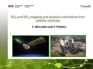
SO 2 and NO 2 mapping and emission estimations from satellite retrievals. C. McLinden and V. Fioletov. Outline. Spatial smoothing, hi-res mapping Air Mass Factor Emission inventories vs. OMI signals Detection of sources, global picture Summary. Satellites measure

E N D
SO2 and NO2 mapping and emission estimations from satellite retrievals C. McLinden and V. Fioletov
Outline • Spatial smoothing, hi-res mapping • Air Mass Factor • Emission inventories vs. OMI signals • Detection of sources, global picture • Summary
Satellites measure vertical column density or number of molecules per cm2 OMI SO2 VCD Mean OMI total column SO2 for Bowen power station with annual emissions of about 170 kT y-1and Belews Creek power station (88 kT y-1)as a function of the distance between the station and the pixel centre. The secondary maximum on the Bowen curve is caused by the contribution of two power plants located about 80 km to the south.
Challenges: Small spatial scales x • Methodologies to better resolve small-scale features in satellite data: • need to use a large amount of data • employ a pixel averaging technique • e.g.: • x= y=4 km, r=20 km • or • x= y=1 km, r=5 km • The value assigned to a gridbox is the average of all data within radius r 40 km y 320 km Mildred Lake r
Pixel Averaging Technique SO2 from OMI, average for 2005-2010 For each grid point of a 2x2 km grid, all overpasses centered within a 12 km from that point were averaged 60 km OMI smallest pixel size 60 km
Air Mass Factors VCDtrop = (SCD – VCDstrat AMFstrat) / AMFtrop • Air mass factor (AMF) describe the sensitivity of the satellite sensor to absorbing layer. They are computed using a multiple-scattering radiative transfer models and their accuracy relies in large part on the validity of input parameters, including: • Shape of the absorbing profile • Surface reflectivity or albedo Spectral Fit Removal of stratosphere Convert Slant to vertical column Tropospheric Vertical Column Density (Level 2) Raw Spectra (Level 0) Calibrated, geolocated Spectra (L1) UV/vis Processing Sequence measured modelled
AMFs and profile shape Altitude-resolved AMF, SZA=60, albedo=0.04 Visible High probability of reaching surface UV Low probability of reaching surface More difficult for UV light to penetrate down to these altitudes due to increased scattering and absorption AMF = AMF’(z) n(z) dz / n(z) dz
Profile Shape June AMF=0.93 OMI NO2 VCD [1015 cm-2] June June AMF = 1.23 VCD [1015 cm-2] GMI global model NO2 - 2 x 2.5
Satellites measure vertical column density In Situ GEOS-Chem or number of molecules per cm2 AQHI research: Innovations using satellite data PM2.5 NO2 MODIS Aerosol Optical Depth Daily OMI Tropospheric Column it can be converted into surface mixing ratio Coincident Model Profile Ground-Level NO2 inferred Lamsal et al., JGR, 2008 Ground-Level PM2.5 van Donkelaar et al., JGR, 2006
OMI NO2 summertime Tropospheric VCD 2005-2010
MODIS aerosol optical depth 2000-2005 Optical Depth
Estimate of emissions • These analyses are used to estimate annual emission rates over local sources • Concept: use accurate, reported emissions from several locations to “calibrate” the satellite observations mass = constant emission rate [tonnes] = [days] [tonnes/day] • Done initially using OMI SO2; will be extended with other species • Constant not universal, additional factors such as windspeed can modify it Interpreted as a “lifetime”
Annual SO2 emissions vs. estimates from a fit of mean OMI SO2 by 2D Gaussian function (2005-2007 data) Fit where R=0.93 Since , a is the total number of molecules. If is in DU, i.e. in 2.69·1026 mol·km-2 , and σx,σy are in km, then a is in 2.69·1026 mol. Mean OMI SO2 Fit Residuals A scatter plot of annual SO2 emission from the largest US sources in 2005 vs. mean OMI SO2 for 2005-2007 integrated around the source estimated using the best fits by 2D Gaussian function. Emissions are given in kT y-1 and molec h-1 units calculated assuming a constant emission rate.
Global SO2 emission source catalogue (~200 sources) Example: Volcanoes in Japan Asama Suwanose-jima Kikai Sakura-jima Aso Miyake-jima
The largest SO2 source in the Arctic: Norilsk, Russia, 70N. Norilsk -1.0 0.0 1.0 2.0 3.0 DU 1% of Russia’s GDP 2% of Russia’s industrial production 3% of Russia’s export … and 2,000,000 T of SO2 per year
Satellite data can be used to track emission changes over time
Cantarell and Ku-Maloob-Zaap Oil Fields, Mexico SO2 2005-2007 Oil production: 800,000+500,000 bpd 2008-2011 OMI estimated SO2 emissions: about 200 kT/y in 2005-2007 about 330 kT/y in 2008-2011
OMI data show a 40% decline in mean SO2 values over Eastern US 2005-2007 2008-2010 The sum of SO2 values from the top 40 emission sources as a function of distance from the source for 2005-2007 (red) and 2008-2010 (blue) Mean OMI SO2 values over the Eastern US for 2005-2007 and 2008-2010. The dots indicate emission sources from the top 40 sources
Oil Sands: OMI monitoring of NO2 emission trends Max VCD • Fit constant + 2D Gaussian to seasonal NO2 VCD data (DJF, MMA, JJA, SON) • Derive trend in total mass (above background) of the enhancement Widths Total mass [t(NO2)] of enhancement Background VCD Maximum VCD Widths of distribution [km] “Background” VCD In-situ NO2 Production [millions of barrels per day]
Summary There is a good correlation between measured OMI SO2 values averaged over a long period and reported emission values. OMI data can be used to monitor sources that emit more than ~70 kT per year. High spatial resolution (a few km) of both measurements and retrieval algorithms is required for emission monitoring