Download

1 / 41
420 likes | 447 Vues
Learn about GIS tools and methods for geologic mapping. Explore different GIS software options and improve your GIS skills through interactive training. Discover tips and techniques for cleaning data, building polygons, and querying spatial information.

E N D
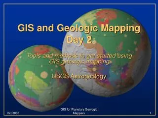
GIS and Geologic MappingPart 2 of 2 Tools and methods to get started using GIS as a base for geologic mapping USGS Astrogeology
GIS-based Mapping • Though this presentation is geared toward geologic mappers, the information is relevant to all GIS users • Screen-shots are likely to differ from individual views • GIS skills are developed through software interaction … be patient and try new things! Tip icon will point out helpful hints throughout the presentation GIS-based Mapping Part 2 (v.1)
An important note. • USGS Astrogeology primarily uses only one “brand” of GIS (ESRI’s ArcMap) • Other brands exist, both free and commercial • “Free” • Quantum GIS (qgis.org/) • UDIG (udig.refractions.net/confluence/display/UDIG/Home) • Open EV (openev.sourceforge.net/) • JUMP (jump-project.org/) • GRASS (grass.itc.it/) • Commercial • TNTmips (www.microimages.com/) • ER Mapper (www.ermapper.com) • PCI GeoMatica (www.pcigeomatics.com) • Global Mapper (www.globalmapper.com) • Integraph (www.intergraph.com) GIS-based Mapping Part 2 (v.1)
GIS Support Nodes • ESRI online portal to technical information • http://support.esri.com • ESRI ArcScripts • http://arcscripts.esri.com/ • ESRI Educational Services • Instructor-led training • Virtual Campus courses • Web workshops GIS-based Mapping Part 2 (v.1)
GIS Support Nodes • Planet-specific information (e.g., data, discussion, tutorials) • http://webgis.wr.usgs.gov/ • USGS discussion board (login required) • http://isis.astrogeology.usgs.gov/IsisSupport/index.php?c=9 “Plugging keywords into a internet search engine is a great way to search for GIS-related assistance!” GIS-based Mapping Part 2 (v.1)
Part 1 Review • Introduced ArcMap & ArcCatalog interfaces • Created a geodatabase (GDB) • Added project-specific attribute domains • Built a Feature Dataset and added three Features (contacts, structures, units) • Imported map bases (raster data) • Edited the Features by adding lines and points (vector data) GIS-based Mapping Part 2 (v.1)
Part 2 Introduction • Cleaning data • Exploring ArcToolbox • Building polygons • Querying data • Calculating spatial statistics “ESRI has on-line tutorials that are helpful in exploring the utility of ArcGIS. Go to www.esri.com and click on the “Training” tab. GIS-based Mapping Part 2 (v.1)
Cleaning data - Cleaning digitized data means improving the appearance of the data by correcting overshoots and undershoots, closing polygons, performing coordinate editing, etc. - paraphrased from ESRI’s online GIS dictionary “Taking time to clean your data as you digitize will help alleviate editing problems and spending excess time near the end of your project.” GIS-based Mapping Part 2 (v.1)
Exercise continued from previous presentation….. Finish contact linework GIS-based Mapping Part 2 (v.1)
Notice that some lines are not connected. To ensure polygons are properly created, all lines must be CLOSED. We need to allow the feature to “snap” to other features. GIS-based Mapping Part 2 (v.1)
Snapping tolerance is the distance at which vertices will connect automatically • Use drop-down to specify unit of measurement • Tolerances are typically project- and scale-specific • “Sticky move tolerance” will allow your pointer to snap to applicable vertices “The editing options dialog box has several changeable parameters such as stream tolerance (the distance between vertices while streaming lines). Try some variations to see what happens!” GIS-based Mapping Part 2 (v.1)
Select line to close • with “select tool” • Choose “Modify Feature” • from ArcEditor Task list GIS-based Mapping Part 2 (v.1)
Snap all lines together in the feature that is being edited. It is easiest to “zoom in” to see where features are not closed. Use the mouse and snap ends together “A topology is a set of rules that constrains how vector data is arranged. Topologies can be used to identify where polyline features are not clean. Use Arc Help for more detail on building and verifying topologies” GIS-based Mapping Part 2 (v.1)
Exploring ArcToolbox • ArcToolbox is an object in ArcMap and ArcCatalog that contains sets of processing tools. Is is presented as a “tree” of tools grouped by functionality. • The toolbox function can be turned on in ArcMap and/or ArcCatalog by clicking on the general menu. “Hovering over menu buttons will provide a short description of the function the button will start” GIS-based Mapping Part 2 (v.1)
ArcToolbox button in ArcMap GIS-based Mapping Part 2 (v.1)
Toolbox window. Close by Clicking the ‘x’ GIS-based Mapping Part 2 (v.1)
Toolbox window • Tools in the toolbox are grouped by similar functions • You can navigate through the tree to see what each does • Toolboxes can be adapted and populated with favorite tools or built for specific projects GIS-based Mapping Part 2 (v.1)
Toolbox window • For example, to add a field to an existing feature, navigate to the “Add Field” tool • Double-clicking will open the tool and provide additional information (see next slide) GIS-based Mapping Part 2 (v.1)
“The “Show/Hide Help” button at the bottom of the tool window will provide helpful information about the tool, required inputs, and options. Explore the toolbox by opening several tools and seeing what they do” GIS-based Mapping Part 2 (v.1)
Building Polygons • Using the toolbox, we can build polygons from our cleaned “contact” polyline feature • Polygons are spatial features that have both area and perimeter • Polygons could represent regions, geologic units, quadrangles, to name a few • Polygons can be built from closed lines “One method of geologic mapping is to build polygons from lines. However, lines can be built from polygons. In such a scenario, polygons are built first, perhaps using the Auto-Complete Polygon editing task. Check it out!” GIS-based Mapping Part 2 (v.1)
Find necessary tool 1. Enter keywords 2. “Click!” • There are >400 tools!!! How do you know where to find the one you need?!?! • Use the “Search” tab and type in some keywords • To find the tool to build polygons, we can type in “polygon” and click “Search” • The “Locate” button will show you where the tool resides on the directory tree 3. Locate the tool GIS-based Mapping Part 2 (v.1)
Find necessary tool • A toolbox search will yield all keyword matches • Open tools that you suspect may be applicable and read the function summary • To build polygons, we will use the “Feature to Polygon” tool GIS-based Mapping Part 2 (v.1)
Populate the dialog box with the necessary information. In our example, we will use “contacts” as the input feature . Notice that we can attribute our new polygons as they are being built by using the “units” point file. “Note the location of the Show/Hide Help button. It is your friend!” GIS-based Mapping Part 2 (v.1)
After some brief computations, the tool process will finish and the newly-created feature will be added to the project. GIS-based Mapping Part 2 (v.1)
Go into the polygon’s properties and change the symbology to use all the populated values for ‘TYPE’. GIS-based Mapping Part 2 (v.1)
Querying the data • GIS empowers the user to perform spatial searches across any or all data within a project • A “query” is “a request to select features or records from a database or feature” • The query expression is typically Boolean (based on yes or no answers) • Queries are commonly performed using a dialog box in ArcMap GIS-based Mapping Part 2 (v.1)
Let’s say that the user wants to find all units that are labeled “plains material”. The user will need to query the data as follows. GIS-based Mapping Part 2 (v.1)
Selecting by feature attributes • Select the layer and field that the query will be based on • “Get Unique Values” will give all values in that field • Build the query and click “OK” GIS-based Mapping Part 2 (v.1)
Selecting by feature location • Features can be selected based on relationships with other features • Examine the “Select by Location” window for specifics GIS-based Mapping Part 2 (v.1)
Calculating Spatial Statistics • A powerful tool to calculate statistics of a zone dataset (e.g., geologic units) based on values from a raster dataset (e.g., elevation) • Spatial Analyst • Cell statistics • Neighborhood statistics • Zonal statistics • Operates out of Spatial Analyst • Right click empty space on tool bar and select “Spatial Analyst” GIS-based Mapping Part 2 (v.1)
Cell Statistics • “A function that calculates a statistic for each cell of an output raster that is based on the values of each cell in the same location of multiple input rasters.” - paraphrased from ESRI’s online GIS dictionary • For example, the user could find the range and maximum value of albedo from multiple overlapping images acquired in different seasons “Spatial Analyst tools such as cell statistics provide critical analytical components for the interpretation of raster and vector data. Statistics can help improve the quality of geologic maps.” GIS-based Mapping Part 2 (v.1)
1 2 3 • 1. Add and/or Remove the raster layers that are required for the statistics • 2. Set the statistic that is required (can be minimum, maximum, range, sum, mean, std dev, variety, majority, minority, median) • 3. Type in the output raster name, either as a temporary file (default - will be erased the next time the project is closed) or as a TIFF, IMG, or Arc GRID. GIS-based Mapping Part 2 (v.1)
Neighborhood Statistics • A function that calculates a statistic on a raster using a user-specified “neighborhood”, which implies an extent from individual cells. The extent can be a annulus, circle, rectangle, or wedge. • The user specifies statistics type, neighborhood extent (e.g., circle with a radius of 4 km), and out output cell size (default-input cell size) • For example, the user could find the range and maximum value of albedo from multiple overlapping images acquired in different seasons “Using Neighborhood Statistics, a user could create a range of filter types. For example, a median high pass filter can be produced by using a median neighborhood statistic and then subtracting the raster value.” GIS-based Mapping Part 2 (v.1)
1 2 3 4 • 1. Determine the input dataset and field that will be the basis of the stats • 2. Set the statistic (minimum, maximum, range, sum, mean, std dev, variety, majority, minority, median) and the neighborhood (annulus, circle, rectangle, wedge) • 3. Set the neighborhood size • Set the output cell size, raster name, and location GIS-based Mapping Part 2 (v.1)
Zonal Statistics • A function that summarizes values in a raster within the zones of another layer • The user specifies the “zone dataset” (e.g., geologic units) the value raster dataset (e.g., slope) • Output is a Table that summarizes zone statistics • For example, the user could find the range and mean value of slope for geologic units “The Zonal Statistics function allows the user to produce a simplified graph of the statistics. Note the check box in the dialog box.” GIS-based Mapping Part 2 (v.1)
1 2 3 • 1. Set the Zone dataset (the feature that contains the region upon which statistics need to be created) • 2. Set the Value raster (the raster dataset that will be the base of the statistics) • 3. Set the statistic that is required (can be minimum, maximum, range, sum, mean, std dev, variety, majority, minority, median) GIS-based Mapping Part 2 (v.1)
Summary • Cleaning data is an important aspect of digitizing vector data • Cleaning can consist of closing gaps, smoothing, removing overshoots (dangles), and verifying projections • ArcToolbox is a suite of tools that is accessible through ArcMap and/or ArcCatalog • ArcToolbox provides a hierarchal tree structure of tools that are grouped by functionality • ArcToolbox can be searched using keywords GIS-based Mapping Part 2 (v.1)
Summary, cont’d • Tools have a “show details” button in the dialog box that provide important details about the tools functionality • There are several stylistic and logistic approaches to building polygons • Polygons can be created from cleaned linework (e.g., build geologic units from geologic contacts) • A point file can be used to attribute newly-created polygon features GIS-based Mapping Part 2 (v.1)
Summary, cont’d • User’s can query their data using either feature attributes or feature locations • Queries are excellent ways to single out pertinent data • Specialized statistics are provided through the Spatial Analyst extension • Spatial statistics can include cell statistics, neighborhood statistics, and zonal statistics GIS-based Mapping Part 2 (v.1)