Download
1 / 68
710 likes | 1.13k Vues
Spatial Solitons 1D. Dissipative Spatial Solitons and Their Applications in Active Semiconductor Optical Amplifiers. Erdem Ultanir, Demetri Christodoulides & George I. Stegeman School of Optics/CREOL, University of Central Florida Falk Lederer and Christopher Lange

E N D
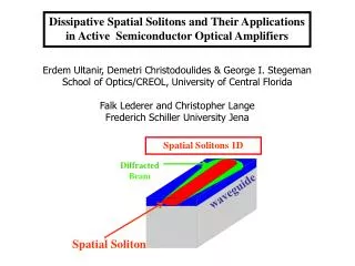
Spatial Solitons 1D Dissipative Spatial Solitons and Their Applications in Active Semiconductor Optical Amplifiers Erdem Ultanir, Demetri Christodoulides & George I. Stegeman School of Optics/CREOL, University of Central Florida Falk Lederer and Christopher Lange Frederich Schiller University Jena Diffracted Beam waveguide Spatial Soliton
Mitchell, White light Soliton (1996) Propagating Spatial Soliton Milestones Picciante, NLC (2000) Bjorkholm, Kerr Solitons in Sat. Media (1974) Duree, Photorefractive (1993) Silberberg, Discrete Array (1997) Barthelemy, 1D Kerr Soliton (1985) Torruellas, 2D Quad. Soliton (1995) 1960 1970 1980 1990 2000 Christodoulides, Discrete (1988) SOA (2002) Segev, Photorefractive Solitons (1992) Chiao & Talanov Prediction of Kerr (1964) Christodoulides, Incoherent (1997) Zakharov, Soliton solutions (1971) Sukhorukov, Prediction of Quadratic Solitons (1975) Akhmediev Cubic-quintic CLGE (1995) • Kerr Solitons, Χ3 effects, integrable system, elastic interactions • Hamiltonian systems (conservative), inelastic interaction, one (or few parameters) • Discrete Hamiltonian systems (includes Kerr) • Dissipative solitons, zero parameter systems
1D Spatial Solitons in Homogeneous Media A spatial soliton is a shape invariant self guided beam of light or a self-induced waveguide Hamiltonian Systems Nonlinearity balances diffraction Non-Hamiltonian (Dissipative Systems) Gain balances loss + nonlinearity balances diffraction No trade-offs in optical beam properties!!
Vp' Self-focusing Spatial Solitons (1+1)D Spatial Solitons (2+1)D phase velocity Vp < Vp' Spatial Solitons inHomogeneousMedia Diffracting beam Planar (slab) waveguide Bulk medium (1+1)D - in a slab waveguide - diffraction in one D (2+1)D - in a bulk material - diffraction in 2D A spatial soliton is a shape invariant self guided beam of light or a self-induced waveguide n2 > 0
Spatial Solitons (1+1)D Spatial Solitons (2+1)D Spatial Solitons inHomogeneousMedia Diffracting beam Planar (slab) waveguide Bulk medium (1+1)D - in a slab waveguide - diffraction in one D (2+1)D - in a bulk material - diffraction in 2D • Soliton Properties: • Robust balance between diffraction and a nonlinear beam narrowing process • Stationary solution to a nonlinear wave equation • Stable against perturbations • Observed and Studied Experimentally to Date in: • Kerr and saturating Kerr media 4. Liquid crystals • Photorefractive media 5. Gain media • Quadratically nonlinear media Semiconductor optical amplifiers n2 > 0
f(x) y Diffraction in 1D Homogeneous System Homogeneous in Diffracting Dimension • Insert into wave equation • Assume slow change over • an optical wavelength
1D Nonlinear Wave Equation depends on nonlinear mechanism Slowly varying phase and amplitude approximation (1st order perturbation theory) nonlinearity diffraction Spatial soliton
x y (2+1)D Kerr solitons are unstable 1D Scalar Kerr Solitons 1 free parameter
Output Intensity 60 40 20 y (microns) 0 -20 Input Power (watts) -40 750 250 500 1D Scalar Kerr Solitons 1 free parameter
Output Light Semiconductor Optical Amplifiers J Top Electrode Input Light J Bottom Electrode • Multi-functional Elements for Optics • 1. Used as optical amplifiers, with feedback as lasers • Used as nonlinear optical devices (mW power levels) • Demultiplexers • All-optical switchers • Wavelength shifters • All-optical logic gates • ….
gain gain z loss loss loss x Freely Propagating Solitons In Gain Systems Self-trapped beams have been observed in SOAs over limited distances G. Khitrova et al., Phys. Rev. Lett. 70, 920 (1993) Hamiltonian diffraction+nonlinearity is balanced Dissipative diffraction+nonlinearity+gain+loss is balanced • Found also in Erbium-doped fibers, laser cavities • Requires intensity dependent • Gain & Loss • Strong attractors
Saturable gain gain Intensity Saturable loss loss gain gain z loss loss loss x Freely Propagating Solitons In Gain Systems • Requires intensity dependent • Gain & Loss • Strong attractors
2w0 N – carrier density Ntr – transparency carrier density gain N' 1 loss Semiconductor Optical Amplifier Modeling Optical field (’) evolution (along z’) G. P. Agrawal, J. Appl. Phys. 56, 3100 (1984) Nonlinear index change Cladding absorption and scattering losses Diffraction Gain h = Henry factor - change index with N ,
N – carrier density Ntr – transparency carrier density Conduction band Valence band Semiconductor Optical Amplifier Modeling Carrier density equation Current Pumping Diffusion Auger Recomb. Field absorption Spontaneous Recomb. Nonradiative Recombination Phonons Generated Optical Beam ,
N – carrier density Ntr – transparency carrier density Semiconductor Optical Amplifier Modeling Carrier density equation Current Pumping Diffusion Auger Recomb. Field absorption Spontaneous Recomb. Nonradiative Recombination Phonons Generated ,
Complex Ginzburg-Landau Equation - For small diffusion ( below) and B=C=0, equations simplify to - Expanding denominator near the bifurcation point Complex Ginzburg-Landau Equation • Solutions in NLO have been investigated systematically by • Nail Akhmediev, Soto-Crespo and colleagues since 1995
- Nonlinear Dynamics: plane wave field solutions have implications for soliton stability • Defining “small signal” gain relative • to transparency point including loss as |Ψo | Supercritical bifurcation Solutions δG Potential For Solitary Wave Solution β, filtering parameter h, linewidth enhancement factor 2bko/a π, pump parameter α, linear loss coefficient
J Top Electrode Input Light Saturable gain gain Output Light J Intensity Bottom Electrode Saturable loss loss Semiconductor Optical Amplifiers The SOA shown above does not support stable plane waves because “noise” experiences larger gain Need to manipulate relative saturable gain and absorption!!
Contact Pads Saturable gain gain Intensity Saturable loss loss solution Stabilizing the Background SOA SA SA SOA SOA SA SOA SA SOA SA
Effect of Controlling Saturable Absorption Versus Gain Saturable gain gain Intensity Saturable loss loss
Stabilizing Background (Plane Waves) Amplifier saturation Unstable background Noncontact region saturation Parameters for Bulk GaAs; D=33 cm2/s, C=10-30 cm6/s, B=1.4x10⁻¹⁰ cm3/s h=3, τ=5x10⁻⁹s, a=1.5x10⁻¹⁶cm2, α=5cm-1
Pumping Current (Amps) Stationary Solutions Unstable Stable Solitons (finite beams) Soliton Bifurcation Diagram gain pumping current ALL soliton properties (width + peak power) determined by current ZERO parameter solitons 10-100 mW power levels
Stationary Solutions ) (10 Intensity Diffraction length Diffraction length Perpendicular axis (cm) Perpendicular axis (cm) Stable Solitons (finite beams) gain pumping current ALL soliton properties (width + peak power) determined by current ZERO parameter solitons 10-100 mW power levels
Etching & Au coating SOA Sample SQW InGaAs 950nm grown in Jena SiN deposition Device fabrication 300μm 11μm 9μm
Single Quantum Well Sample SQW InGaAs
Average system equation Carrier densities in gain,absorption sections (1) (2) (3) SQW Modelling QW modeling Parameters; D. J. Bossert, Photon. T. Lett. 8, 322 (1996)
Steady state intensity and phase distribution 20μm Phase radians Gaussian beam excitation Intensity Positionμm ) (10 Intensity Diffraction length Diffraction length Perpendicular axis (cm) Perpendicular axis (cm) Propagating Solitons Current pumping small signal gain Soliton peak intensity and width Zero Optical Parameter System -
100A max, Pulsed Diode Driver 500ns/500Hz (0mW-200mW) I Ti sapphire (CW) 910-970nm CCD camera BS 40x 20x λ/2 Cylindrical Telescope 1cmX800μm Patterned SOA at 21.5 oC OSA Input Output (@965nm, I=0) ~1 μm Sample defects 15.2μm FWHM 60.7μm FWHM ~4 diffraction lengths
100A max, Pulsed Diode Driver 500ns/500Hz (0mW-200mW) I Ti sapphire (CW) 910-970nm CCD camera BS 40x 20x λ/2 Cylindrical Telescope 1cmX800μm Patterned SOA at 21.5 oC OSA Output (@950nm, I=4A) Input ~1 μm 15.5μm FWHM 15.2μm FWHM ~4 diffraction lengths
Unstable Output Profile vs Intensity Change Experiment Current (amps) Position μm Stable solitons BPM Simulations (10cm) X Subcritical branch Position μm Input Power (mW)
Unstable Output Profile vs Current Change Experiment Current (amps) Position μm Stable solitons BPM simulations Position μm Subcritical branch Current (A)
m) μ Output FWHM ( Input beam waist FWHM ( μ m) Soliton Properties I=4A (b) Experiment Too few soliton periods Diffraction dominated (c) Solitons (d) Solitons Position μm Solitons are zero parameter
Soliton Properties 946nm, 15.9μm 941nm, 39.3μm Solid line g=104cm-1, h=3; dashed dotted line g=60cm-1, h=3; dashed line g=60cm-1, h=1
J Periodic Electrode Input Light Output Light J Bottom Electrode Periodically Patterned Semiconductor Optical Amplifier • Periodic regions of gain and absorption. • 2. Absorption region saturates before gain • 3. Stable “autosoliton” with gain=loss • For given pumping current J, soliton power • & width fixed (zero parameter soliton family) • Soliton has a strong phase chirp • 10-100 mW power levels
Do Multi-Component Dissipative Solitons Exist? • In Kerr (n=n2I systems “Manakov” solitons exist and are stable! • Simplest case is two orthogonal incoherent polarizations - AlGaAs at 1.55 m n2 same for both TE and TM, and n2 = n2 - coherence between TE and TM eliminated by passing through different dispersive optics - Manakov solitons have 1. Spatial width independent of polarization ratio 2. No energy exchange between polarizations Spatial width invariant for TE/TM = 0.1 10
Experimental Setup • 2 Orthogonally polarized Beams • Different Wavelengths from 2 Different Lasers • Mutually Incoherent Beams Grating to separate beams at different wavelengths TS – tunable wavelength and power, titanium sapphire laser operated at =943nm LD – laser diode, very limited temperature tunability, operated at =946nm, 40mW power
Conclusions • There are no completely stable, multi-component dissipative solitons in this case • The two beams form quasi-stable solitary waves over cm distances which depend on input power • 3. Even though optical beams are incoherent, they do interact for by competing for excited carriers in order to compensate for loss • Although the wavelengths are almost identical, the gain, loss etc. coefficients are slightly different! • Similar results found by using the quintic complex Ginzburg-Landau equation
n1 n2 > n1 Collisions Between Coherent Solitons light bent (drawn) into region of higher refractive index Solitons in phase Solitons out of phase Other phase angles Energy Exchange
K : = 0 S : = 0 K, S : = K, S : = 0 K, S : = 3/2 K, S : = /2 Collisions Between Coherent Solitons - relative phase between solitons K - Kerr Nonlinearities S - Saturating Nonlinearities
Non-local nonlinearity Output channels 20μm Intensity Phase radians A B C D Positionμm -0.58 Δn (x10-4) Gain cm-1 100μm 4.09 100μm - - 8.77 Positionμm Soliton Interactions • Possibilities • Gates • Beam scanners • Modulation of one output • with optical input • etc,…
Non-local nonlinearity Output channels 20μm Intensity Phase radians A B C D Positionμm -0.58 gain gain Δn (x10-4) Gain cm-1 100μm 4.09 100μm - z loss loss loss - 8.77 x Positionμm Soliton Interactions
Beam scanner Output 1 Output 2 22μm 15.3μm Input 2 *exp(jΦ(t)) Input 1 Dissipative Local Interactions Parallel excitation 3 1.5 Propagation Distance Propagation length cm 0 0 200 -200 Position μm Position μm
Dissipative Non-Local Interactions I Input2 *exp(jΦ(t)) Input1 51μm output1 output2 50μm
Center sees different waveguide Gain cm-1 1cm 8mm 6mm 4mm 2mm Position m Dissipative Non-Local Interactions II Output 2 Output 1 66μm 70μm Input 1 Input 2 *exp(jΦ(t))
Center sees different waveguide Simulation Phasediff = 0 Phasediff = π 3 3 2 2 Propagation distance (cm) 1 1 0 0 - 100 - 50 0 50 100 - 100 - 50 0 50 100 Position μ m Position μ m Experiment Dissipative Non-Local Interactions II Output 2 Output 1 66μm 70μm Input 1 Input 2 *exp(jΦ(t))
Input2 *exp(jΦ(t)) Input1 56μm output1 output2 46μm Dissipative Non-Local Interactions III Simulation Experiment