Download

1 / 42
420 likes | 612 Vues
Quantitative Data Analysis: Univariate (cont’d) & Bivariate Statistics. Neuman and Robson Chapter 11. Research Data library at SFU http://www.sfu.ca/rdl/. Class Session Activities. Quiz 2 More on Univariate Statistics Begin Bivariate Statistics If time:

E N D
Quantitative Data Analysis: Univariate (cont’d) & Bivariate Statistics Neuman and Robson Chapter 11. • Research Data library at SFU • http://www.sfu.ca/rdl/
Class Session Activities • Quiz 2 • More on Univariate Statistics • Begin Bivariate Statistics • If time: • Hans Rosling on Using Empirical Research to Understand World Change http://www.youtube.com/watch?v=hVimVzgtD6w • Hans Rosling: “Let my data set change your mind set” http://www.youtube.com/watch?v=KVhWqwnZ1eM&feature=related
Recall: Univariate Statistics • Frequency distributions: explore each variable in a data set, separately to see the pattern of responses • Measures of central tendency of the values (mean, median, mode) • Measure of variation or variation(range, percentile, standard deviation, z-scores)
Studying Frequency Distributions • Raw Data Obtain a printout of the raw data for all the variables. • resembles a matrix, with the variable names heading the columns, and the information for each case or record displayed across the rows. Source (for next examples): http://www.csulb.edu/~msaintg/ppa696/696uni.htm
Example: Raw data for a study of injuries among county workers (first 10 cases) Raw data is difficult to grasp, especially with large number of cases or records.
To present the information in a more organized format, start with univariate descriptive statistics for each variable. Example: The variable “Severity of Injury”
Frequency Distribution for “Severity of Injury” • Obtain a frequency distribution of the data for the variable. • Identify the lowest and highest values of the variable, • Put all the values of the variable in order from lowest to highest. • count the number of appearance of each value of the variable. This is a count of the frequency with which each value occurs in the data set.
Grouped Data • Decide on whether the data should be grouped into classes. • Example: The severity of injury ratings can be collapsed into just a few categories or groups. • Grouped data usually has from 3 to 7 groups. • There should be no groups with a frequency of zero (in this example, there are no injuries with a severity rating of 7 or 8). • Ways to construct groups: • equal class intervals (e.g., 1-3, 4-6, 7-9). • Approximately equal numbers of observations in each group. • Remember that class intervals must be both mutually exclusive and exhaustive.
Caution: Grouping Response Categories • To make new categories • Facilitate analysis of trends • But decisions have effects on the interpretation of patterns
Cumulative Frequency Distributions • include a third column in the table (this can be done with either simple frequency distributions or with grouped data • How many injuries were at level 5 or lower? Answer=7
Percentaged Frequency Distributions • Frequencies can also be presented in the form of percentage distributions and cumulative percentagescumulative percentages
Why Graph? • way of visually presenting data • present the data • summarize the data • enhance textual descriptions • describe and explore the data • make comparisons easy • avoid distortion • provoke thought about the data
Bar Graphs (Bar Charts) • to display frequency distributions for variables measured at the nominal & ordinal levels. • use the same width for all the bars with space between bars. • label the parts of the graph, including the title, the left (Y) or vertical axis, the right (X) or horizontal axis, and the bar labels.
Histograms • for interval and ratio level variables • width of the bar is important, since it is the total area under the bar that represents the proportion of the phenomenon accounted for by each category • bars convey the relationship of one group or class of the variable to the other(s).
Histogram example • In the case of the counties & employee injuries, we might have information on the rate of injury according to the number of workers in each county in State X.
Grouping Categories (Histograms) • If we group injury rates into three groups: • low rate of injury would be 0.0-1.9 injuries per 1,000 workers; • moderate would be 2.0-3.9; • high would be 4.0 and above (in this case, up to 5.9).
Frequency Polygon • another way of displaying information for an interval or ratio level variable. • also used to show time series graphs, or the changes in rates over time.
Pie Chart • Another way to show the relationships between classes or categories; • each "slice" represents the proportion of the total phenomenon that is due to each of the classes or groups.
Another visual representation of a distributions: Pie charts
Bivariate Statistics (relations between 2 variables) • After examining univariate frequency distribution of the values of each variable separately, • To study joint occurrence & distribution of the values of the independent and dependent variable together. • The joint distribution of two variables is called a bivariate distribution.
Contingency Tables (Cross-tabulations) • A contingency table shows the frequency distribution of the values of the dependent variable, given the occurrence of the values of the independent variable. • Both variables must be grouped into a finite number of categories (usually no more than 2 or 3 categories) such as low, medium, or high; positive, neutral, or negative; male or female; etc.
Features of Contingency Table • Title • Categories of the Independent Variable head the tops of the columns • Categories of the Dependent Variable label the rows • Order categories of the two variables from lowest to highest (from left to right across the columns; from top to bottom along the rows). (Usually but not always). • Show totals at the foot of the columns
Basic Terminology (Tables) • Parts of a Table • title (conventions) • Order of naming of variables • Dependent, independent, control • body, cell, column, row • “marginals” • sources, date
Constructing a Contingency Table • if the variables not divided into categories, decide on how to group the data. • obtain a frequency distribution for the values of the independent variable; • obtain a frequency distribution for the values of the dependent variable • obtain the frequency distribution of the values of the dependent variable, given the values of the independent variable (either by tabulating the raw data, or from a computer program • display the results of step 4 in a table
Table 1. Attitudes toward Consolidation by Area of Residence Interpreting a Contingency Table • Inspect the contingency table for patterns. (difficult if there are different totals of observations in the different categories of the independent variable)
Interpreting a Contingency Table • Convert the observations in each cell to a percentage of the column total; • be sure to still show the total number of observations for each column on which the percentages are based. (N= total number per column) • Compare the percentages across the categories of the dependent variable (the rows).
Percentaged Contingency Table (example)Table 1b: Attitudes toward Consolidation by Area of Residence
Interpreting a Contingency TableTable 1. Attitudes toward Consolidation by Area of Residence • more city residents (54%) than non-city residents (37%) are for consolidation. Conversely, more non-city residents (39%) than city residents (19%) are against consolidation. About the same percentage of both groups have no opinion about Description: More city residents (54%) than non-city residents (37%) are for consolidation. Conversely, more non-city residents (39%) than city residents (19%) are against consolidation. About the same percentage of both groups have no opinion about consolidation.
Grouping categories (Collapsing categories) U.N. example Babbie, E. (1995). The practice of social research Belmont, CA: Wadsworth
Collapsing Categories & omitting missing data Babbie, E. (1995). The practice of social research Belmont, CA: Wadsworth
Types of Relationships or Associations between two variables • Correlation (or covariation) • when two variables ‘vary together’ • a type of association • Not necessarily causal • Can be same direction (positive correlation or direct relationship) • Can be in different directions (negative correlation or indirect relationship) • Independence • No correlation, no relationship • Cases with values in one variable do not have any particular value on the other variable
What is an association between two variables? • Can the value of one variable be predicted, if we know the value of the other variable? • Example: half the people participating in training programs get a job. What is the likelihood of any one participant getting a job? About fifty-fifty. So we would not be very good at predicting whether people will get jobs or not. • If we introduce a second variable (i.e. length of time in training), does it help us to be more accurate in our predictions of the likelihood that someone will get a job?
Two variables • Dependent variable: Obtaining a Job No job=100 Gets a job=100 • Independent Variable: Length of Training Program Short=100 Long=100
Bivariate Distribution--Perfect Positive Relationship(If training is good for getting a job) If we know the length of the training program, we can perfectly predict the likelihood of getting a job. The longer the training program, the more likely the participant is to get a job and, conversely, the shorter the training program the less likely the participant is to get a job.
Bivariate Distribution--Perfect Inverse Relationship • If we know the length of the training program, we can perfectly predict the likelihood of getting a job. The longer the training program, the less likely the participant is to get a job and, conversely, the shorter the training program the more likely the participant is to get a job. That is, as the training program length increases, likelihood of obtaining a job decreases.
Bivariate Distribution--No Relationship • (If training has no relationship with getting a job) 50/50 guess. Knowing the length of the training program does not help to predict the likelihood of getting a job.
Techniques for examining relationships between two variables • Cross-tabulations or percentaged tables • Graphs, scattergrams or plots • Measures of association (e.g. correlation coeficient, etc.)
Interpreting a Relationship between two variables • Do the patterns in the tables mean that there is a relationship between the two variables (in example: area of residence and attitude toward consolidation)? • Is one's attitude about consolidation associated with one's area of residence? • If there is a relationship, how strong is it? Are the results statistically significant? Are the results meaningfully significant? • In order to answer these questions, we must turn to a set of statistics called Measures of Association (next day).