On-line Parallel Tomography
On-line Parallel Tomography. Shava Smallen UCSD. Talk Outline. I) Introduction to On-line Parallel Tomography II) Tunable On-line Parallel Tomography III) User-directed application-level scheduler IV) Experiments V) Conclusion. What is tomography?.

On-line Parallel Tomography
E N D
Presentation Transcript
On-line Parallel Tomography Shava Smallen UCSD
Talk Outline I) Introduction to On-line Parallel Tomography II) Tunable On-line Parallel Tomography III) User-directed application-level scheduler IV) Experiments V) Conclusion
What is tomography? • A method for reconstructing the interior of an object from its projections • At the National Center for Microscopy and Imaging Research (NCMIR), tomography is applied to electron microscopy to study specimens at the cellular and subcellular level
Example Tomogram of spiny dendrite (Images courtesy of Steve Lamont)
Parallel Tomography at NCMIR projection scanline • Embarrassingly parallel Z specimen slice X Y projection scanline
Off-line parallel tomography (off-line PT) Data resides somewhere on secondary storage Single, high quality tomogram Reduce turnaround time Previous work (HCW’ 00) On-line parallel tomography (on-line PT) Data streamed from the electron microscope long makespan, configuration errors, etc. Iteratively computed tomogram Soft real-time execution NCMIR Usage Scenarios
On-line PT • Real-time feedback on quality of data acquisition • ) First projection acquired from microscope • ) Generate coarse tomogram • ) Iteratively refine tomogram using subsequent projections (refresh) • Update each voxel value • Size of tomogram is constant
NCMIR Target Platform • Multi-user, heterogenous resources • NCMIR cluster • SGI Indigo2, SGI Octane, SUN ULTRA, SUN Enterprise • IRIX, Solaris • Meteor cluster • Pentium III dual proc • Linux, PBS • Blue Horizon • AIX, Loadleveler, Maui Scheduler network
On-line PT Architecture ptomo slices tomogram ptomo ptomo scanlines ptomo projection ptomo writer preprocessor
On-line PT Design 1) Frame on-line parallel tomography as a tunable application • Resource limitations / dynamic • Availability of alternate configurations [Chang,et al] • each configuration corresponds to different output quality and resource usage 2) Coupled with user-directed application-level scheduler (AppLeS) • adaptive scheduler • promote application performance
On-line PT Configuration • Triple: (f, r, su) • Reduction factor (f) • Reduce resolution of data reduce both computation and communication • Projections per refresh (r) • Reduce refinement frequency reduce communication • Service Units - (su) • Increase cost of execution increase computational power
User Preferences • Best configuration (f, r, su) = (1, 1, 0 ) • Several possible configurations user specifies bounds • projections should be at least size 256x256 • 1 f 4 or 1 f 8 • user could tolerate up to a 10 minute time wait • 1 r 13 • reasonable upper bound • 0 su (50 x acquisition period x c)
User-directed reduction factor projections per refresh service units • Feasible? • Use dynamic load information • if work allocation found • Better? • e.g. 1. (1, 6, 4) - best f 2. (2, 2, 8) - good su/r 3. (2, 1, 20) - best r
User-directed AppLeS generate request process infeasible adjust request request feasible display triples review rejects all triples accepts one find work allocation User-directed AppLeS User execute on-line PT
Triple Search • Search parameter space • If triple satisfies constraints feasible • Constrained optimization problem based on soft real-time execution • compute constraint • transfer constraint • Heuristics to reduce search space • e.g. assume user will always choose (1,2,1) over (1,2,4)
Work Allocation cpu availability work allocation compute constraints processor availability transfer constraints ptomo-to-writer bandwidth subnet-to-writer bandwidth cost user constraints Multiple mixed-integer programs approx soln
Experiments • Impact of dynamic information on scheduler performance • Usefulness of tunability Grid environments • Scheduling latency
Dynamic Information • We fix the triple and let schedulers determine work allocation
Simulation • Evaluate schedulers • Repeatibility • Long makespan • several resource environments • Simgrid (Casanova [CCGrid’2001]) • API for evaluating scheduling algorithms • tasks • resources modeled using traces • E.g. Parameter sweep applications [HCW’00] • Simtomo
Performance Metric expected refresh period actual refresh period relative refresh lateness • Relative refresh lateness
NCMIR experiments 4:00 pm 8:00 am • Traces (8 machines) • 8 hour work day on March 8th, 2001 • Ran simulations throughout day at 10 minute intervals
Perfect Load Predictions 4 10 wwa wwa+cpu wwa+bw AppLeS 3 10 mean relative refresh lateness 2 10 1 10 0 10 0 1 2 3 4 5 6 7 8 hours since 3/8/2001 - 8:00 PST
Imperfect Load Predictions Student Version of MATLAB
Synthetic Grids • Bandwidth predictibility • Average prediction error • pi {L, M, H} • p1 p2 p3 • e.g. LMH • 27 types • 2510 Grids x 4 schedulers • 10,040 simulations p1 p3 p2
Relative Scheduler Performance 705.89 658.91 127.10 1.07 Student Version of MATLAB
Partial Ordering • Performance vs. bandwidth predictability • Grid predictibility • Partial orders using p1 p2 p3 • Comparable/Not Comparable • e.g. HML is comparable to HLL • e.g. HLM is not comparable to LHM • HHH, HHM, HMM, HLM, MLM, LLM, LLL
Example Partial Order 4 10 wwa wwa+cpu wwa+bw AppLeS 3 10 relative refresh lateness (seconds) 2 10 1 10 0 10 HHH HHM HMM HLM MLM LLM LLL .
Tunability Experiments • How useful is tunability? • variability • Fixed topology • categorized traces • L, M, H • v1 v2 v3 v4 v5 • 243 Grid types v4 v1 v5 v3 v2
Tunability Experiments 4 x 10 6 4 su 2 0 15 10 8 6 5 4 2 0 0 r f • Run over a 2 day period • back-to-back • assume single user model • f, r, su • Set of triples chosen • T = {1,…,61}
Tunability Results 1 f r 0.9 su 0.8 0.7 0.6 fraction of changes 0.5 0.4 0.3 0.2 0.1 0 parameters • Count how many times a triple changed per 2-day simulation • e.g. • 12.9% • 25.7%
Scheduling Latency 7000 6000 5000 4000 number of experiments 3000 2000 1000 0 0 2 4 6 8 10 seconds • Time to search for feasible triples • e.g. • 88% under 1 sec • 63% under 1 sec
Conclusions and Future Work • Grid-enabled version of on-line parallel tomography • Tunable application • Tunability is useful in Grid environments • User-directed AppLeS • Importance of bandwidth predictability • e.g. rescheduling • Scheduling latency is nominal • Production use