Simulating Large Networks with a Fluid Flow Model: Techniques and Applications
This paper discusses a fluid flow model developed for simulating large-scale networks, collaboratively researched by Yong Liu and colleagues. It covers methodologies for solving ordinary differential equations (ODEs), including considerations for network topology and computation savings. The model integrates with packet-level simulators to examine TCP flows and provides a detailed analysis of active queue management strategies. Key topics include TCP congestion control mechanisms, random early detection (RED), and adjustments made to ensure accurate simulation outcomes, addressing various challenges and open issues in network simulation.

Simulating Large Networks with a Fluid Flow Model: Techniques and Applications
E N D
Presentation Transcript
Simulating Large Networks using Fluid Flow Model Yong Liu Joint work with Francesco LoPresti, Vishal Misra Don Towsley, Yu Gu
Outline • Fluid Flow Model • ODE solving Methods • Account for Topology • Computation Savings • Model Adjustments • Integration with Packet Level Simulators • Open Issues
Fluid Model of a Network of AQM Routers Supporting TCP Flows Routers within network drop/mark packets when buffers fill up TCP runs at the “edge” network
TCP Congestion Control: window algorithm • Window: can send W packets at a time • increase window by one per RTT if no loss • decrease window by half on detection of loss
receiver W sender TCP Congestion Control: window algorithm Window: can send W packets • increase window by one per RTT if no loss • decrease window by half on detection of loss
receiver W sender TCP Congestion Control: window algorithm • Window: can send W packets • increase window by one per RTT if no loss • decrease window by half on detection of loss
Active Queue Management:RED • RED: Random Early Detect proposed in 1993 • Proactively mark/drop packets in a router queue probabilistically to • Prevent onset of congestion by reacting early • Remove synchronization between flows
- q (t) -x (t) t -> The RED Mechanism RED: Marking/dropping based on average queue length x (t) (EWMA algorithm used for averaging) 1 Marking probability p pmax tmin tmax 2tmax Average queue length x x(t): smoothed, time averaged q(t)
Modeling RED: A Single Congested Router • One bottlenecked AQM router • service capacity {C (packets/sec)} • queue length q(t) • drop prob. p(t) • N TCP flows • window sizes Wi (t) • round trip time Ri (t) = Ai+q (t)/C • throughputs Bi(t) = Wi (t)/Ri (t) TCP flowi,prop. delayAi AQM router C, p
Additive increase Mult. decrease Loss arrival rate Queue length: Outgoing traffic Incoming traffic System of Differential Equations All quantities are average values. Timeouts and slow start ignored Window Size:
p x System of Differential Equations (cont.) Average queue length: Where a= averaging parameter of RED(wq) d= sampling interval ~ 1/C Loss probability: Where is obtained from the marking profile
Stepping back: Where are we? W=Window size, R = RTT, q = queue length, p = marking probability N+2 coupled equations solved numerically
Fluid Flow Model for a Network with Multiple Bottle-necks Network of M RED queues, K TCP classes, flows in class k Scalable with link bandwidth and flow population within each class
ODE Solving Methods • Matlab ODE Solver Suit • Error control, automatically adjusted step-size • Cannot handle delayed differential equations • Lack of flexibility of programming • Computational Inefficiency • Fixed Stepsize Runge-Kutta Method • FFM: Time stepped numerical fluid model solver in C
Computation Cost: Matlab vs. FFM 80 TCP Classes x 20 RED Queues, Random Routing Matrix FFM: 5 seconds Matlab: 1572 seconds
Accuracy: FFM vs. NS Single Bottle Neck Network, 2 TCP Classes, Flows Per Class: 60 40 20
Account for Topology Fact: TCP sending rate will be reshaped in each queue it traverses C C Q2 Q1 Packet Loss Probability (I) Packet Loss Probability (II)
Account for Topology Keep track of each TCP class’s arrival rate and departure rate at each queue:
Account for Topology FFFM: Finer Fluid Flow Model Packet Loss Probability (I) Packet Loss Probability (II)
Model Adjustment 1 In ns, actual packet drop/mark prob. is not equal to loss probability calculated from RED formula. Given a RED calculation value p, RED tries to make the interval between two drops/marks uniformly distributed in [1/p, 2/p] when “wait” option is on and [1, 1/p] when “wait” is off. Actual loss prob. is 2p/3 if “wait” on; 2p if “wait” off
Model Adjustment 1 With wait: Without wait:
Model Adjustment 2 NS won’t drop packet if the queue is empty Adjustment:
Other Adjustments • TCP Newreno and SACK only backoff once for multiple losses • within one window. • Adjustment 1: • Adjustment 2: • At a given time, only TCP flows without packet loss will increase their congestion window.
NS vs. FFFM {1,2} {1}{1,2,3}
NS vs. FFFM (cont.) 3 TCP Classes, 8 RED Queues Class1 Class3 Class2 Scale bandwidth and flow population with k=1, 10, 50. Link Bandwidth: (black) 100M*k, (red) 10M*k Flows within each class: 40*k
TCP Average Sending Rate, K=1 Class1 Class2 Class3
Queue Length, K=1 Bottle-neck2 Bottle-neck1
TCP Average Sending Rate, K=10 Class2 Class1 Class3
Queue Length, K=10 Bottle-neck1 Bottle-neck2
TCP Average Sending Rate, K=50 Class1 Class2 Class3
Queue Length, K=50 Bottle-neck1 Bottle-neck2
TCP Average Sending Rate, K=100 Class1 Class2 Class3
Queue Length, K=100 Bottle-neck1 Bottle-neck2
1.2 0.2 1.0 1.3 Net 1 Net 0 1.4 0.0 0.1 1.1 1.5 4 5 2.0 2.1 3.0 3.1 Net 3 Net 2 2.2 2.3 3.2 3.3 Topology of a Large IP Network
Integration with Packet Level Simulators Simulated by FFFM Packet Level Packet Level Fluid flow model can provide delay and loss information for packets passing fluid network segments. If traffic from packet segments is negligible to fluid segment, fluid model can be solved independently.
Integration into NS FFFM has been integrated into NS by constructing Fluid Link and Fluid Network objects. Fluid Network Fluid Network Segment Access Access Access Ns node Ns node Ns node Packet Network Segment Topology of Hybrid NS Simulation
Hybrid NS Simulation Link Bandwidth: (black) 100M, (red) 15M 3 Background TCP Classes, 40 Flows per Class 3 Foreground TCP Sessions Fluid Network Segment Class2 Class1 Class3 Session3 Session1 Session2 Packet Level Nodes
Background TCP Average Window Size Class1 hybrid packet Class2 Class3
Foreground TCP Sample Path Session1 Session2 Session3
Bottle-neck Queue Evolution Bottle-neck1 Bottle-neck2 Simulation time: Hybrid: 8.4s, Packet: 29.7s CPU: 800MHz, Memory: 256M
Open Issues • Time-out, Slow Start • Finite duration flows, unresponsive flows • High interaction between packet network segments and fluid network segments • Limitations of mean value fluid model • Verify results for large networks