Introduction to Interferometric Synthetic Aperture Radar - InSAR
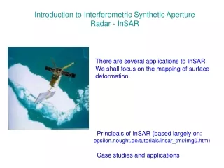
Introduction to Interferometric Synthetic Aperture Radar - InSAR. There are several applications to InSAR. We shall focus on the mapping of surface deformation. Principals of InSAR (based largely on: epsilon.nought.de/tutorials/insar_tmr/img0.htm) Case studies and applications.


Introduction to Interferometric Synthetic Aperture Radar - InSAR
E N D
Presentation Transcript
Introduction to Interferometric Synthetic Aperture Radar - InSAR There are several applications to InSAR. We shall focus on the mapping of surface deformation. • Principals of InSAR (based largely on: epsilon.nought.de/tutorials/insar_tmr/img0.htm) • Case studies and applications
First Acquisition (Master) Second Acquisition (Slave) 5.56 mm Master Slave Df r1 r2 Dr Change in LOS
If: Earth was flat. The satellite orbit was fixed. No atmosphere. Then: Things were simple, and the calculation of ground deformation would have been indeed an easy task. In practice, however, in order to obtain the deformation field, it is necessary to perform quite a few corrections.
Viewing Position Spherical Earth Topography Deformation Atmosphere
SAR is an active sensor Unlike passive sensors, the SAR transmits a signal and measures the reflected wave. So the SAR can “see” day-and-night. The signal wave length was selected such that its absorption by atmospheric molecules is minimal. ERS
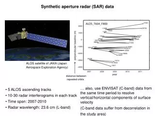
SAR geometry ERS1/2 azimuth range Launch date: ERS1 July 1991 ERS2 April 1995 Altitude: 780 km Incidence angle: 23 degrees Period: 100 minutes Repeat time: 35 days
Orbit geometry Polar (almost) orbit Ascending and descending Ground tracks Ascending track Descending track
The (SAR) data The SAR records the amplitude and the phase of the returned signal amplitude phase Mt. Etna Image from http://epsilon.nought.de/tutorials/insar_tmr/img35.htm Note that while the amplitude image shows recognizable topographic pattern, the phase image looks random.
The phase The phase is mostly due to the propagation delay, but also due to coherent sum of contributions from scatters within the resolution element. Figure from Rosen et al., 2000
The phase The phase is proportional to the two-way travel distance divided by the transmitted wavelength.
InSAR geometry The baseline, B, is the orbit separation vector. Baselines should be less than 200 meters, and the shorter the better!
InSAR processing: amplitude coregistration The two images, i.e. the “slave” and the “master”, do not overlap. So we need to figure out which group of pixels in the “slave” corresponds to which group of pixels in the “master”. This is done through cross-correlating sub-areas in the two images. This step requires a huge number of operations, and is by far the most time consuming step in the process. Image from http://epsilon.nought.de/tutorials/insar_tmr/img38.htm
InSAR processing: phase interferogram Calculate phase interferogram, i.e. subtract the phase of of the “slave” from that of the “master”. phase “master” phase interferogram phase “slave” - = Note that while both the master and slave appear random, the interferogram does not.
InSAR processing: flat-earth removal Next, we need to remove the phase interferogram that would result from a flat-earth. - = After removing the flat-earth effect we are left with an interferogram that contains topography+deformation between the two acquisitions and atmospheric effect.
InSAR processing: Remove topographic phase Height of ambiguity: the amount of height change that leads to a 2 change in interferometric change:
InSAR processing: Remove topographic phase (cont.) The longer the baseline, the smaller the topographic height needed to produce a fringe of phase change (or, the longer the baseline is the stronger the topographic imprint). Image from http://epsilon.nought.de/tutorials/insar_tmr/img17.htm
InSAR processing: unwrapping The interferogram is a map of an ambiguous phase offset between - and +. In order to recover the absolute unambiguous phase offset, one needs to unwrap the data. Phase unwrapping is a tricky business, here’s one algorithm: Image from http://epsilon.nought.de/tutorials/insar_tmr/img27.htm
While the wrapped phase looks like this: The unwrapped phase looks like this: * Note that in this specific example the topographic effect has not been removed, thus the unwrapped phase map correspond mainly to topographic height.
InSAR processing: geocoding This final step amounts to mapping the phase from satellite to geographic coordinates. latitude azimuth range longitude Figure from: http://earth.esa.int/applications/data_util/SARDOCS/_icons/c2_SAR_geo2.jpg
The seismic cycle: Figure from: Wright, 2002.
Seismic displacement: The utilization of SAR data to map surface deformation started with the ground-breaking study of the 1992 Landers earthquake in California [Massonnet et al., 1993]. Massonnet, D., M. Rossi, C. Carmona, F. Adragna, G. Peltzer, K. Feigl, and T. Rabaute, The displacement field of the Landers earthquake mapped by radar interferometry, Nature, 364, 138-142, 1993.
Seismic displacement (cont.): It is hard to unwrap the interferogram, if the deformation is discontinuous. In such cases, it is convenient to present the results in wrapped form. Yellow-red-blue : target moved a way from the satellite. Red-yellow-blue : target moved towards the satelite. Figure from: http://www.eorc.jaxa.jp/ALOS/gallery/images/5-disaster/obs-geometry5.gif
Seismic displacement (cont.): It turned out that the crust is an elastic half-space! 4 Dec. 1992, Magnitude 5.1, near Landers - CA
Seismic displacement (cont.): Magnitude 5.6 from Western Iran. Processed and calculated by Maytal Sade
Seismic displacement (cont.): The 1999 Izmit earthquake in Turkey [Wright et al., 2001]
Seismic displacement (cont.): The 1999 Izmit earthquake in Turkey [Wright et al., 2001] Modeling the data helps to: Constrain the rupture geometry and co-seismic slip distribution. Identify triggered slip.
Seismic displacement (cont.): The 1999 Izmit earthquake in Turkey [Wright et al., 2001]
Seismic displacement (cont.): The displacement field projected onto a map view may be obtained by using both the ascending and the descending tracks. In order to go beyond the 2D displacement field, an additional information should be incorporated -the azimuth offset. The 3-D displacement field in the area of 1999 Hector Mine in California (Fialko et al., 2001): The 3 equations: The 3 unknowns:
Inter-seismic displacement: Obviously, resolving co-seismic (large) deformation is easier than resolving inter-seismic (small) deformation. The signal to noise ratio may be amplified by stacking multiple interferograms (the more the better). Application of the stacking approach to NAF (Wright et al., 2001): Because inter-seismic strain accumulates steadily with time, the contribution of each pair is scaled proportionally to the interval between acquisitions.
Inter-seismic displacement (cont.): Figure from Wright et al., [2001, GRL] A recipe for reducing atmospheric contribution: It is useful to form interferogram chains in such a way that each date is used as a master the same number of times it is used as a slave. The atmospheric effect of these acquisitions is exactly canceled out, and we are left only with the atmospheric contribution from the start and the end of the chain (see Holley, 2004, M.Sc. thesis, Oxford).
Earthquake location: Locating small-moderate quakes in southern Iran (Lohman and Simons, 2005): Figure from Pritchard, 2006, Physics Today