Download
1 / 40
400 likes | 623 Vues
Examination of Quantum Gravity Effects with Neutrino. Alexander Sakharov. John Ellis, Nicholas Harries, Nick Mavromatos, Anselmo Meregaglia, Andre Rubbia, Sarben Sarkar. Discrete ‘ 08, December 12, Valencia. Outlook. Lorentz violation in neutrino propagation.

E N D
Examination of Quantum Gravity Effects with Neutrino Alexander Sakharov John Ellis, Nicholas Harries, Nick Mavromatos, Anselmo Meregaglia, Andre Rubbia, Sarben Sarkar Discrete ‘ 08, December 12, Valencia
Outlook Lorentz violation in neutrino propagation Manifestation of quantum gravity for «low» energy radiation probe Limits on LV from Supernovae neutrino signals • Neutrino emission from a SN • Optimisation of dispersive broadened neutrino signal CNGS and OPERA experiment Quantum gravity decoherence in neutrino oscillations Quantum deoherence • MSW – like effect induced decoherence • Stochastic fluctuations of space-time background Sensitivity of CNGS and J-PARC beam to QG decoherence
I Lorentz violation in neutrino propagation
In the approximation , the distortion of the standard dispersion relation may be reresnted as an expansion in Modification of dispersion relation The existence of the lower bound at which space-time responses actively to the present of energy, may lead to violation of Lorentz invariance. Linear deviation Quadratic deviation
Liouville strings (J. Ellis, N. Mavromatos, D. Nanopoulos, 1997, 1998, 1999) • Effective field theory approach (R.C. Mayers, M. Pospelov 2003) • Sace-time foam (L.J. Garay 1998) • Loop quantum gravity (R. Gambini, J. Pullin, 1999) • Noncomutative geometry (G. Amelino-Camelia, 2001) • Fermions-neutrinos (J. Ellis, N. Mavromatos, D. Nanopoulos, G.Vlkov, 1999) • Gravitationally brain localized SM particles (M.Gogberashvii, et al, 2006)
At the source At the detector E2 E2 < E1 E1
GRBs neutrino-photon ::, D beyond 7000 Mpc(Piran, Jakob,2006) Photons Pulsars: E up to 2GeV, D about 10 kpc,(Kaaret, 1999) GRBs::E up to MeV, D beyond 7000 Mpc(Ellis, et al, 2005,2007) AGNs::E up to 10 TeV, D about 100s Mpc(MAGIC and Ellis, et al , 2007) Neutrinos SN: E about 10 MeV, D about 10 kpc,(Ellis, et al, 1999; Ammosov and Volkov, 2000 ) MINOS:: , D=734 km(MINOS, et al, 2007)
Energy release of 10th of MeV neutrinos is consistent with the expected A future galactic supernova is expected to generate events in SK Neutrino emission from Supernovae About 20 neutrinos from SN1987a in LMC were detected by KII, IMB and BAKSAN During the later stage (after neutronization peak) all flavors are produced with Fermi-Dirac spectra Oscillations in the core are taken into account
Any other (“incorrect”) would spread in time the events The “correct” value of should always compress the neutrino signal Minimal dispersion (MD) Event list with low number of events with no a reasonable time profile to be extracted
SN 1987a Minimal Dispersion
Energy cost function (ECF) The apparent duration of a pulse is only going to be increased by dispersion. The energy per unit time decreases with the distance from the source. The dispersion can be figured out by "undoing" the dispersion such that as much energy as possible is emitted at the source.
(t1,t2) contains the most active part of the flare, as determined using KS statistics One corrects for given model of photon dispersion, linear and quadratic, by applying to each photon of energy E the time shifts.
Future Galactic Supernova Energy Cost Function Super-Kamiokande
Each individual bunch has a duration of CC events expected to be observed in the 1.8 kton OPERA CNGS beam characteristics The average neutrino energy: Extraction the SPS beam during spills of length Within each spill, the beam is extracted in 2100 bunches separated by
Spill analysis 100ns uncertainty in the relative timing
Slicing estimator Estimate the mean arrial times of 1000-event slice with increasing energies Straight line fit Straight line fit
Comparing two histograms, namly a referece one and with shifts itroduced OPERA may also be used to measure the timing of muons from neutrino events in the rocks Rock Events Distortion of the shape of the spill at its adges
Bunch analysis If a sub-ns resolution in OPERA coud be acchived If a synchronization of the SPS and OPERA clocks with ns precision over period 5 years could be obtained !!Challenging task!!(free electrol lasers with 10th picoseconds pulses- synchronisation over several km) To survive the bunch periodic structure
Conclusions I SN 1987a: Future SN: CNGS spill: CNGS bunch structure: CNGS bunch structure (rocks):
II Quantum gravity decoherence in neutrino oscillations
Quantum decoherence The time evolution of a closed quantum system Pure state Mixed state Space-time foam environment (Ellis, et al, 1984) Nonunitary evolution (Lindblad mapping) H with stochastic element in a classical metric Generically space-time foam and the back-reaction of matter on the gravitational metric may be modeled as a randomly fluctuating environment
MSW-like effect Foam medium is assumed to be to be described by Gaussian random variable The average number of foam particles (Maromatos and Sarkar, 2006) The modified time evolution (master equation)
Stochastic fluctuations of Space-Time metric backgrounds 1+1, no spin - random variables - plane wave solution of KG equation - dispersion relation
- covariance matrix for random variables average over the stochastic space-time fluctuations - combined time evolution
Lindblad-type (F. Benatti and R. Floreanini, 2001) No energy dependence Inversely proportional to energy Proportional to energy squired
Gravitational MSW No energy dependence Proportional to energy
Modify the standard oscillation formula including damping factors • Generate fake data with standard neutrino oscillation formula • Calculate 2 • Qualitatively, we observe both the spectral distortion and suppression in the number of events, if there is decoherence, in addition to the conventional oscillations
CNGS CERN-SPSOPERA L=732 km<E>=17 GeV; 4.5£ 1021 pot/year5 years2kT photo-emulsion Measure spectrum by reconstructing from CC events
J-PARC Tokay SK L=295 km<E>=600 MeV; 1.0£ 1021 pot/year5 years T2K-22.5 kT water cherenkov Measure spectrum by reconstructing single- Cherenkov- ring QE and non-QE events Near detector Maximal oscillation point Off axis 20 T2KK 100 kT Argon
Atmospheric Solar + KamLand (E. Lisi, A. Marrone and D. Montanino, 2000; Fogli, et al, 2007)
Concluding remarks • CNGS and J-PARC beams are very sensitive, in some particular cases, to QG induced decoherence effects • In principle, the problem to distinguish between different dependences of damping exponents can be resolved it there are two baselines • Damping signatures could be mimicked by uncertainties in determination of neutrino energy and propagation length • Long baseline experiments are less affected by the risk of erroneous misinterpretations of conventional effects as a signature of decoherence
Synchronization GPS discipline oscillations (GPSDO) “Common-view” GPS, the same GPS satellite for CERN and LNGS clock “Carrier-Phase” GPS, carrier frequency instead of the codes transmitted by the satellite Optical timing synchronization
Common View GPS Time Transfer Two stations, A and B, receive a one-way signal simultaneously from a single transmitter and measure the time difference between this received signal and their own local clock Each station observes the time difference between its clock and GPS time plus a propagation delay, which can be largely removed by using the one-way GPS time transfer procedures. By exchanging data files and performing a subtraction, the time difference between the two receiving stations is obtained and the GPS clock drops out The accuracy of common-view time transfers is typically in the 1 to 10 ns range
CNGS J-PARC T2K
Since in practice neutrino wave is neither detected nor produced with sharp energy of well-defined propagation length, we have to average over theL/Edependence etc
pessimistic optimistic
Atmospheric GNGS