Sampling Distributions
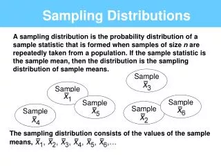
Sampling Distributions. What is a sampling distribution?. Grab a sample of size N Compute a statistic (mean, variance, etc.) Record it Do it again (until all possible outcomes are recorded or infinitely) The resulting distribution is a sampling distribution Articulation of the Sample Space.


Sampling Distributions
E N D
Presentation Transcript
What is a sampling distribution? • Grab a sample of size N • Compute a statistic (mean, variance, etc.) • Record it • Do it again (until all possible outcomes are recorded or infinitely) • The resulting distribution is a sampling distribution • Articulation of the Sample Space
Concept of the Effect Size • Related to Study Outcome • Indicates relations between X and Y (relations between IV and DV) • Indicates magnitude of effect • Size of effect, Effect Size
Two Common Effect Sizes • Correlation, r • Standardized Mean Difference, d
ES Sampling Distributions • If delta = 0, distribution approx normal • If rho = 0, distribution approx normal • If not zero, distributions are not normal. Customary to apply fixes for this (discussed later).
Empirical (Monte Carlo) Sampling Distributions • Examine R programs • In running R, you will want to save your outputs in separate files that let you keep records. The graph is replaced (overwritten) each time you run a graphical command • Form groups and complete exercise
You need to input parameters. You don’t need to understand the computations unless you want to write your own programs. Some results show here; others in a separate window shown on additional slides.
Results of running the sim (histogram) N = 120; rho = .8
Results of running the sim (boxplot) N = 120; rho = .8
You input the parameters. If you start with a standardized mean difference (e.g., d = 1), you can just set one mean to zero, the other to the value of d, and the standard deviations within each group to 1.0. The program is written to give you more flexibility (e.g., you can see what happens if the variances and sample sizes are unequal across groups).
d = 1 N1=N2=15 (M1=14 M2=15) (SD1 = SD2 =1)
d = 1 N1=N2=15 (M1=14 M2=15) (SD1 = SD2 =1)
Exercise 3a • What happens to the standard error of the mean (square root of the sampling variance) of r as rho increases from near zero to near 1 • (use rho = 0, .3, .6, .9, • samplesize=100, • Nsamples=10000 • What happens to the shape of the sampling distribution of r (particularly skew) as rho increases from near zero to near 1 • (use the same values for the simulation)? • Create a table and an illustrative graph or series of graphs to tell your story. Prepare to present to the class.
Exercise 3b • What happens to the standard error of the mean of d as delta increases? • Use delta= 0, .5, 1, 2 (use SD=1 and choose means) • N1=N2=25 • Nsamples = 100000 • What happens to the shape of the sampling distribution of d as delta increases (use the same values)? • Create a table and an illustrative graph or series of graphs to tell your story. Prepare to present to the group.