Download
1 / 29
290 likes | 376 Vues
Explore David Mumford's insights on image modeling for computer vision, focusing on scaling properties, kurtosis, natural images, and the analysis of image statistics. Discover the potential of textons, wavelets, and primitives in creating realistic images.

E N D
What is the ‘right’ mathematical model for an image of the world? 2nd lecture David Mumford January, 2013 Sanya City, Hainan, China
Many sorts of signals are understood so well we can synthesize further signals of the same ‘type’ not coming from their natural source. • Speech is close to this except the range of natural voices has not been well modeled yet. • BUT natural images, images of the real world are far from being accurately enough modeled so we can synthesize images of ‘worlds that might have been’. • I believe this is a central question for computer vision. It is a key to Grenander’s ‘Pattern Theory’ program. • You cannot analyze an image when you have no idea how to construct random samples from the distribution of potential real world scenes.
Outline of talk • The scaling property of images and its implications: model I • High kurtosis as the universal clue to discrete structure: models IIa and IIb • The ‘phonemes’ of images • Syntax: objects+parts, gestalt grouping, segmentation • PCFG’s, random branching trees, models IIIa and IIIb • Parse graphsand the problem of context sensitivity.
1. Scaling properties of image statistics “Renormalization fixed point” means that in a 2Nx2N image, the marginal stats on an NxNsubimage or an averaged NxN image should be the same. In the continuum limit, if ‘random’ means a sample from a measure μon the space of Schwarz distributions D′ (R2), then scale-invariant means
Evidence of scaling in images: horizontal derivative of images at 4 dyadic scales. There are many such graphs. The old idea of the image pyramid is based on this invariance. Vertical axis is log of probability; dotted lines = 1 standard deviation. Curves vertically displaced for clarity
The sources of scaling The distance from the camera or eye to the object is random. When a scene is viewed nearer, all objects enlarge; further away, they shrink (modulo perspective corrections). Note blueberry pickers in the image above.
A less obvious root of scaling • On the left, a woman and dog on a dirt road in a rural scene; on the right, enlargement of a patch. • Note the dog is the same size as the texture patches in the dirt road; and in the enlargement, windows and shrub branches retreat into ‘noise’. • There is a continuum from objects to texture elements to noise of unresolved details
Model I: Gaussian colored noisescale invariance spectrum 1/f 2 Looks like clouds. Scale invariance implies images like this one cannnot be measurable functions!! Left: 1/f3 noise – a true function. Right: white noise, equal power in all freq.
2. Another basic statistical property -- high kurtosis • Essentially all real valued signals from nature have kurtosis (=μ4/σ4) greater than 3 (their Gaussian value). • Explanation I: the signal is a mixture of Gaussians with multiple variances (‘heteroscedastic’ to Wall Streeters). Thus random mean 0 8x8 filter stats have kurtosis > 3, and this disappears if the images are locally contrast normalized. • Explanation II: a Markov stochastic process with i.i.d increments always has values Xt with kurtosis ≥ 3, and if >3, it has discrete jumps. (Such variables are called infinitely divisible). Thus high kurtosis is a signal of discrete events/objects in nature.
Huge tails are not needed for a process to have jumps: generate a stochastic process with gamma increments
The Levy-Khintchine theorem for images If a random ‘natural’ image I is a vector valued infinitely divisible variable, then L-K applies, so: • The Ik were called ‘textons’ by Julesz, are the elts of Marr’s ‘primal sketch’. • What can we say about these elementary constituents of images? • Edges, bars, blobs, corners, T-junctions? • Seeking the textons experimentally – 2x2, 3x3 patches :Ann Lee, Huang, Zhu, Malik, …
Levi-Khinchine leads to the next level of image modeling • Random natural images have trans. and scale-invariant stats • This means the primitive objects should be ‘random wavelets’: Model IIa • Must worry about UV and IR limits – but it works. • A complication: occlusion. This makes images extremely non-Markovian, leads to the ‘Dead Leaves’ (Matheron, Serra) or ‘random collage’ model (Ann Lee): Model IIb
4 random wavelet images with different primitives Abstract art? Top images by YannGousseau; Morel and Gousseau have sythesized ‘paintings’ in many artists’ styles
3. In search of the primitives: equi-probable contours in the joint histograms of adjacent wavelet pairs (filters from E.Simoncelli, calculation by J.Huang) Bottom left: horizontally adjacent horizontal filters. The diagonal corner illustrates the likelihood of contour continuation; the rounder corners on the x- and y- axes are line endings. Bottom right: horizontally adjacent vertical filters. The anti-diagonal elongation comes from bars giving a contrast reversal; the rounded corners on the axes comes from edges making one filter respond but not the other. These cannot be produced by products of an independent scalar factor and a Gaussian.
Image ‘phonemes’ obtained by k-means clustering on 8x8 image patches Thesis of J. Huang J. Malik: “It’s always edges, bars and blobs!”
Ann Lee’s study of 3x3 patches Take all 3x3 patches, normalize mean to 0, take those with top 20% contrast, normalize contrast: result is a data-point on S7. In this 7-sphere, perfect edges form a surface E. Plot the volume in tubular neighborhoods of E and the proportion of data-points in them. There is a huge concentration around E with asymptotic infinite density.
4. Grouping laws and the syntax of images • Our models are too homogeneous. Natural world scenes tend to have homogeneously colored/textured parts with discontinuities between them: this is segmentation. • Is segmentation well-defined? NEARLY if you let it be hierarchical and not one fixed domain decomposition, allowing for the scaling of images. Larger objects are made up of parts and parts have yet smaller details on them.
3 images from the Malik database, each with 3 human segment-ations
Segmentation of images is sometimes obvious, sometimes not: clutter is a consequence of scaling The classic mandrill: it segments unambiguously into eyes, nose, fleshy cheeks, whiskers, fur My own favorite for total clutter: an image of log driver in the spring timber run. Logs do not form a consistent texture, background trees have contrast reversal, snow matches white water.
The gestalt school formalized some of the complex ways primitives are grouped into larger objects(Metzger, Wertheimer, Kanisza,…) • Elements of images are linked on the basis of: • Proximity • Similar color/texture These are the factors used in segmentation • Good continuationThis is studied as contour completion • Parallelism • Symmetry • Convexity • Reconstructed edges and objects can be amodal as well as modal:
The best way to model the hierarchy of objects and parts and their grouping is by a grammars. Grammars on not unique to language but are ubiquitous in structuring all thought. They have two key properties: • Re-usable parts: parts which reappear in different situations, with modified attributes but their essential identity the same • Hierarchy: these re-usable parts are grouped into bigger re-usable parts which also reappear, with the same subparts. The bigger piece has slots for its components, whose attributesthat must be consistent.
5. The simplest grammars are built from random branching trees • Start at the root. Each node decides to have k children with probability pk, where Σpk= 1. Continue infinitely or until no more children. • λ= Σkpkis the expected # of children; if λ≤1, then the tree is a.s. finite; if λ>1, it is infinite with positive probability • Can put labels, from some finite set L, on the nodes and make a labelled tree from a prob. distr. which assigns probabilities to a label {l} having k children with labels {l1,..., lk}. • This is identical to what linguists call PCFG’s (=probabilistic context-free grammars). For them, L is the set of attributed phrases (e.g. ‘singular feminine noun phrases’) plus the lexicon (nodes with no children) and the tree is assumed a.s. to be finite.
To make an image from the tree, the nodes of the tree correspond to subsets of the image domain; the labels tell you what sort of primitive occurs there.
A model to parse a range of human bodies with a random branching tree (Marr; Rothrocket al)
Graft random branching trees into the random wavelet model • Seed scale space with a Poisson process (xi,yi,ri) with density Cdxdydr/r3. • Let each node grow a tree with growth rate <(r/r0)2. • Put primitives on seeds, e.g. face, tree, road. It passes attributes to its children, e.g. eyes, trunk, car. • Combine by adding or with occlusion – models IIIa/b.
6. But we need context sensitive grammars Children of children need to share information, i.e. context. This can be done by giving more and more attributes to each node to pass down. This theory is being developed by Song-Chun Zhu and Stuart Geman. Here are two examples – a face and a sentence of a 2 ½ yr. old
A parse graph has • a node for each subset of the signal that is naturally grouped together • A vertical edge when one subset contains or a horizontal edge if it is adjacent to another. • Productions: rules for expanding a node into parts. • Ex: the letter ‘A’ with four hierarchical levels • Pixels • Disks tracing medial axis of strokes • Complete strokes and background • Complete letter
Illustrating levels of constraints imposed by context (Zhu et al) A stochastic grammar based model for clock faces in which constraints are successively added.
Are we done? • Far from it. • Learning and fitting grammars to images is a very active area. We need shapes of many kinds, textures, symmetries, occlusion – but thetre seems to be no basic obstacle. • How complex a grammar do we need (think the movie Avatar or the range of styles of abstract art)? • How far can you get with 2D models when the world is 3D? • Good luck.