Download
1 / 17
180 likes | 437 Vues
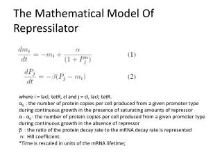
The Mathematical Model Of Repressilator. where i = lacl , tetR , cl and j = cl , lacl , tetR . α 0 : the number of protein copies per cell produced from a given promoter type during continuous growth in the presence of saturating amounts of repressor

E N D
The Mathematical Model Of Repressilator where i = lacl, tetR, cl and j = cl, lacl, tetR. α0 : the number of protein copies per cell produced from a given promoter type during continuous growth in the presence of saturating amounts of repressor α - α0 : the number of protein copies per cell produced from a given promoter type during continuous growth in the absence of repressor β : the ratio of the protein decay rate to the mRNA decay rate is represented n: Hill coefficient. *Time is rescaled in units of the mRNA lifetime;
Augmented Model (Using NR to solve the steady state solutions): • Initial implementation: • Discretized differential equations of protein and mRNA concentration (equation 3 -4). • Requirements for the protein and mRNA has desired oscillation periods(equation 5-6). • Requirements for the reaction rates that they should be independent of the time. (equation 7) where K = (α, β, α 0, n).
Difficulty Using NR To Solve The System Equations • The steady state solutions are strongly dependent on the initial guess. • The size of discretization need to be large, like 75 points, otherwise the solutions we get are not accurate enough.
Modified Augmented Model (Using DSODE to Solve the Concentrations and Reaction Rates) The following set of equation can be solved using DSODE solver After acquiring the protein, mRNA concentrations and the computed reaction rates, Pi(t = 0) − Pi(t = T) = εpi and mi(t = 0) − mi(t = T) = εmican be set up as parameters to check whether the computed reaction rates can lead to oscillations with desired period, T . ε is used to check the variability of the computed reaction rates after acquiring the solutions to the above equations using DSODE.
Wrong Results of Modified Augmented Model and the Reasons Protein and mRNA concentrations Time (mRNA lifte time) Figure 1: red dots represent that epsilon < 0.01 *2 *Amplitude. Amplitude=(maximum-minimum)/2. Figure 2: The protein and mRNA concentrations vs. time. • The reason lead to the wrong results are due to the following fact: • The change of protein concentration after time T (desired period) , pi(t=0)-pi(t=T), depends on the actual slope of protein concentration vs. time graph.
Wrong Results of Modified AgumentedModel and the Reasons-Continue Suppose period T=55 is the desired period and the change of protein concentration need to be evaluate. For the green colored protein, if the starting point is set at t=3, then the protein concentration at t=59 need to be tested. If a different starting point of the same green protein was set, like t=5, the relative change is: Protein and mRNA concentrations Time (mRNA lifte time) Figure 2: The protein and mRNA concentrations vs. time. The relative change of the protein concentration is strongly depends on the starting points. In such case, the fixed threshold set up in the model can blocks out some of the right answers and keep some of the wrong answers. For example, if the solution is near the bottom of the waveform where the slope is not big, the relative change of the protein concentration is small and it can not be sort out by the threshold.
Alternations • If the relative change of the protein concentration at the peak of the wave of each types of protein and mRNA can be used, the previous problem can be fixed. • Then if the peak of the wave of each types of protein and mRNA can be successfully found, the period of the system can be found too. • An alternative way can be used to find the reaction rate spaces is to find the period of the oscillation system.
Finding the Period • After acquiring the concentration of the protein and mRNA with time, the period can be computed by find the time difference between the two adjacent peaks or bottoms. • After obtained the period, the threshold can be set up as: ε=(Tactual-Tdesired )/Tdesired • Then the reaction rate spaces with different values of period can be obtained.
Reaction Rate Spaces by Finding the Period Two- Dimension reaction rate space projections. Tdesired= 42 mRNA life time Figure 2: Threshold ε= (Tactual − Tdesired)/Tdesired. The yellow, cyan, red, blue and black dots represent ε < 1%, 5%,10%,20%, > 20%.
Checking the Viability of the Computed Reaction Rates Tdesired = 42 mRNA life time Figure 4: protein concentration vs. time
Two- Dimension Reaction Rates vs. Periods Projections Tdesired = 42 mRNA life time Figure 5: Threshold ε= (Tactual − Tdesired)/Tdesired. The yellow, cyan, red, blue and black dots represent ε < 1%, 5%,10%,20%, > 20%.
Reaction Rate Spaces by Finding the Period Two- Dimension reaction rate space projections. Tdesired = 42 mRNA life time Figure 6: Threshold ε= (Tactual − Tdesired)/Tdesired. The yellow, cyan, red, blue and black dots represent ε < 1%, 5%,10%,20%, > 20%. The green dots on both graphs behave strange because the actual period is longer than the computed time length, so there is no computed period returned.
Two- Dimension Reaction Rates vs. Periods Projections Tdesired = 42 mRNA life time Figure 7: Threshold ε= (Tactual − Tdesired)/Tdesired. The yellow, cyan, red, blue and black dots represent ε < 1%, 5%,10%,20%, > 20%. The green dots on both graphs behave strange because the actual period is longer than the computed time length, so there is no computed period returned.
Reaction Rate Spaces by Finding the Period Tdesired = 42 mRNA life time Two- Dimension reaction rate space projections. Figure 8: Threshold ε= (Tactual − Tdesired)/Tdesired. The yellow, cyan, red, blue and black dots represent ε < 1%, 5%,10%,20%, > 20%. The green dots on both graphs behave strange because the actual period is longer than the computed time length, so there is no computed period returned.
Two- Dimension Reaction Rates vs. Periods projections Tdesired = 42 mRNA life time Figure 9: Threshold ε= (Tactual − Tdesired)/Tdesired. The yellow, cyan, red, blue and black dots represent ε < 1%, 5%,10%,20%, > 20%. The green dots on both graphs behave strange because the actual period is longer than the computed time length, so there is no computed period returned.
Physical Range Of The Period • In DSODE, the code run 80000 steps. The first 30000 steps are used to insure that there are no damping oscillations. The next 50000 steps are used to find the period. These 50000 steps correspond to 100 mRNA life time. • The total run time is very important since with different reaction rates, the period is different. For example, if β is small, the period will be big. If the run time is too small, one complete period will not be computed. But if the period is too large, it might outside the physical range and do not need to be considered.
Long Range Damping Oscillation • Al though the code has run enough time, it still might be some small damping. Will it still be considered as an oscillation?