Mathematical Model

1. AN INTERACTIVE POSSIBILISTIC LINEAR PROGRAMMING APPROACH FOR MULTIPLE OBJECTIVE TRANSPORTATION PROBLEMSDr. Celal Hakan Kagnicioglu, Assistant Anadolu UniversityESYO Yunusemre Kampusu 26470 Eskisehir/TURKEYTel:00-90-222-3351775e-mail: chkagnic@anadolu.edu.tr

2. Transportation problem(TP) is an important linear programming that includes many applications such as job scheduling, production inventory, production planning, production distribution, allocation problems and investment analysis. • Efficient algorithms have been developed for solving the transportation problem when the cost coefficients and the supply and demand quantities are known exactly.

3. However, these parameters are not always in a precise manner. The unit shipping cost may vary in a time frame can be an example of it. The supplies and demands may be uncertain due to some uncontrollable factors. • Due to incompleteness and/or unavailability of required data over the mid-term decision horizon, critical parameters ( such as transportation cost and demand ) are assumed to be imprecise in nature.

4. To deal quantitatively with imprecise information in making decisions, Bellman and Zadeh(1970) and Zadeh(1978) introduce the notion of fuzziness. • Since the transportation problem is essentially a linear program, fuzzy linear programming techniques are applied to the fuzzy transportation problem.

5. This paper deals with solution of the multiple objective transportation problems by an interactive possibilistic linear programming approach. • In this transportation problem, there are two objective functions which are • Minimization of transportation cost and • Minimization of transportation time. • Transportation costs, demand and supply are fuzzy coefficients with triangular possibility distribution. • Transportation times are assumed to be crisp in the model.

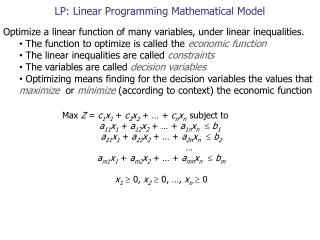
6. Mathematical Model Minimize Zk = , k=1,2,…,K subject to , i =1,2,…,m, , j =1,2,…,n, for all i and j. The decision variable Xij represents the quantity to be transported from origin Oi to destination Dj. The sources can be production facilities and the destinations can be warehouses, and at each origin Oi let ai be the amount of a homogenous product transported to n destinations Dj to satisfy the demand for bj units of the product there. A penalty Cij is associated with transporting a unit of the product from origin i to destination j.

7. Interactive possibilistic linear programming model Minimize Z1 = Minimize TT =

8. 1 ΠC Figure1.The triangular possibility distribution of • The most pessimistic value (Cp) that has a very low likelihood of belonging to the set of available values (possibility degree = 0 if normalized) • The most possible value (Cm) that definitely belongs to the set of available values (possibility degree = 1 if normalized) • The most optimistic value (Co) that has a very low likelihood of belonging to the set of available values (possibility degree = 0 if normalized) Cp Cm Co C

9. Fuzzy objective with a triangular possibility distribution can be converted into three crisp objectives. This objective can be minimized by pushing the three points toward the left. Solving the fuzzy objective becomes the process of minimizing zp, zm and zo simultaneously. However, there may exist a conflict in the simultaneous optimization process. By using Lai and Hwang’s approach, zm and (zo-zm) are minimized and (zm-zp) is maximized, rather than simultaneously minimization of zp, zm and zo. That is, this approach simultaneously minimizes the most possible value of the imprecise total costs, zm, maximizes the possibility of obtaining lower total costs, (zm-zp), and minimizes the risk of obtaining higher total costs, (zo-zm).

10. Min Z1 = Zm = • Max Z2 = Zm - Zp = • Min Z3 = Zo - Zm = • Min Z4 = TT =

11. 1 Min Zm ΠZ Max (Zm-Zp) Min (Zo-Zm) . Zp Zm Zo Figure 2.The strategy to minimize the total costs This auxiliary multiobjective linear programming problem can be solved by converting into an equivalent single goal linear programming problem by using the Zimmermann’s (1978) fuzzy programming method. At first, the positive ideal solutions (PIS) and negative ideal solutions (NIS) of the three objective functions should be obtained: Z1(Pis)= Min Zm, Z1(Nis)= Max Zm Z2(Pis)= Max ( Zm- Zp ), Z2(Nis)= Min ( Zm - Zp ) Z3(Pis)= Min ( Zo- Zm ), Z3(Nis)= Max ( Zo- Zm ) Z4(Pis)= Min TT, Z4(Nis)= Max TT.

12. . The linear membership function of these objective functions f1(3)(Z1(3))=f2(Z2)= . If the minimum acceptable possibility, β, is given, then the auxiliary crisp equality constraints can be presented as follows: İ=1,2,…m j=1,2,….n

13. Finally, after having the crisp constraints for the TP, Zimmerman’s equivalent single objective linear programming model is applied to obtain the overall satisfaction compromise solution. Max L s. to L ≤ f1(Z1) L ≤ f2(Z2) L ≤ f3(Z3) L ≤ f4(Z4) i =1,2,…,m, j =1,2,…,n. 0 ≤ L ≤ 1, Xij ≥ 0 for all i and j, where fi (Zi) is the satisfaction degree of the ith objective function.

14. Algorithm The algorithm for solving the TP is as follows. • Model the imprecise coefficient and right-hand sides of the formulated multiobjective TP model using triangular possibility distribution. • Three new crisp objective functions for the imprecise objective function is developed. These three new objective functions minimize the most possible total cost value, maximize the possibility of obtainin lower costs and minimize the risk of obtaining higher costs, respectively. • Given the minimum acceptable possibility, β, imprecise constraints are converted into crisp ones by the weighted average method. • After having PIS and NIS of the objective functions separately, linear membership functions are specified for all the objective functions, and then the auxiliary multiobjective TP is converted into an equivalent linear programming model by the method of Bellman and Zadeh (1970) and Zimmermann’s (1978) fuzzy programming method. • The model is solved and linear membership function is modified interactively until the solution is satisfactory. When the solution is accepted as satisfactory, it is stopped.

15. W1 W2 W3 W4 W5 W6 Supply PF1 (20,25,28) (28,33.36) (19,23.25) ……….. (35,37,40) PF2 (13,16.20) (9.12.16) (18,22,25) ……………… (62,64,67) PF3 (36,38,39) (23,25.26) (14,16,19)………………. (38,40,41) PF4 (64,66,70) (37,40,44) (45,47,50)………………. (37,39,40) PF5 (44,46,50) (25,28,31) (46,49,53)…………….… (40,43,45) PF6 (67,69,73) (23,26,28) (33,36,38)…………….… (22,24,28) Demand(20,24,26) (55,60,63) (17,19,22)………………. Table1. Transportation costs, supply and demand data All values are imprecise numbers with triangular possibility distributions. Transportation time (minute) of a product from production facilities to warehouses are precise values.

16. Transportation problem is formulated according to the multiobjective linear programming model described above. • The imprecise data is modeled by triangular possibility distributions. There are two objective functions of the model • Three new crisp objective functions are developed for the imprecise objective function. Therefore, the model has four objective functions. • Since right-hand side of the constraints (demand and supply) are imprecise, auxiliary crisp constraints are formulated by using weighted average method at β = 0.5. • Four crisp objective functions of the auxiliary multiobjective linear programming problem presented in the example are solved using the crisp single-goal linear programming model

17. According to these solutions, the corresponding PIS and NIS of the initial solutions are specified. • By using different set of PIS and NIS of the objective functions, the corresponding linear membership function of all the objective functions can be defined. • Two different set of PIS and NIS values are used for the solutions

18. Since transporatation cost (Z1)is imprecise and has a triangular possibility distribution, it is calculated by (Z1 – Z2, Z1, Z1 + Z3). • Therefore, the initial transportation cost is imprecise and has a triangular possibility distribution of ( 5599.9, 6368.0, 6841.1 ), and transportation time (Z4), is 8191.0 minutes. • The improved solution is also imprecise and has a triangular possibility distribution of ( 5338.5, 6147.9, 6749.5 ), and transportation time is 8288.8 minutes. • Overall satisfaction degree of the objectives increased from 0.44 to 0.70 by the improved solution.

19. Since TP is not balanced (supply = demand) due to imprecise values, the number of products transported in the improved solution ( ∑xij = 228.7 ) is greater than in the initial solution ( ∑xij =220.6 ). • Changes in the PIS and NIS of the objective functions are very effective on the value of the overall satisfaction degree of the objectives (L).

20. CONCLUSION This approach helps to solve most of the real life transportation problems with multiobjective and imprecise and precise parameters through an interactive decision making process. This work aims to present an interactive possibilistic linear programming problem approach for solving multiobjective transportation problems with imprecise cost, demand and supply. By this approach, simultaneously the most possible value of the imprecise total costs are minimized, possibility of obtaining lower total costs are maximized and, the risk of obtaining higher total costs are minimized.