Image Classification using Attribute Classifiers for Shopping Websites
Train and classify web shopping images based on color attributes. Enhance e-commerce browsing experience with accurate image classification.

Image Classification using Attribute Classifiers for Shopping Websites
E N D
Presentation Transcript
Classification Tamara Berg CSE 595 Words & Pictures
HW2 • Online after class – Due Oct 10, 11:59pm • Use web text descriptions as proxy for class labels. • Train color attribute classifiers on web shopping images. • Classify test images as to whether they display attributes.
Topic Presentations • First group starts on Tuesday • Audience – please read papers!
Example: Image classification input desired output apple pear tomato cow dog horse Slide credit: Svetlana Lazebnik
http://yann.lecun.com/exdb/mnist/index.html Slide from Dan Klein
Example: Seismic data Earthquakes Surface wave magnitude Nuclear explosions Body wave magnitude Slide credit: Svetlana Lazebnik
The basic classification framework y = f(x) • Learning: given a training set of labeled examples{(x1,y1), …, (xN,yN)}, estimate the parameters of the prediction function f • Inference: apply f to a never before seen test examplex and output the predicted value y = f(x) output classification function input Slide credit: Svetlana Lazebnik
Some classification methods Neural networks Nearest neighbor 106 examples LeCun, Bottou, Bengio, Haffner 1998 Rowley, Baluja, Kanade 1998 … Shakhnarovich, Viola, Darrell 2003 Berg, Berg, Malik 2005 … Conditional Random Fields Support Vector Machines and Kernels Guyon, Vapnik Heisele, Serre, Poggio, 2001 … McCallum, Freitag, Pereira 2000 Kumar, Hebert 2003 … Slide credit: Antonio Torralba
Example: Training and testing • Key challenge: generalization to unseen examples Training set (labels known) Test set (labels unknown) Slide credit: Svetlana Lazebnik
Classification by Nearest Neighbor Word vector document classification – here the vector space is illustrated as having 2 dimensions. How many dimensions would the data actually live in? Slide from Min-Yen Kan
Classification by Nearest Neighbor Slide from Min-Yen Kan
Classification by Nearest Neighbor Classify the test document as the class of the document “nearest” to the query document (use vector similarity to find most similar doc) Slide from Min-Yen Kan
Classification by kNN Classify the test document as the majority class of the k documents “nearest” to the query document. Slide from Min-Yen Kan
Classification by kNN What are the features? What’s the training data? Testing data? Parameters? Slide from Min-Yen Kan
Decision tree classifier Example problem: decide whether to wait for a table at a restaurant, based on the following attributes: • Alternate: is there an alternative restaurant nearby? • Bar: is there a comfortable bar area to wait in? • Fri/Sat:is today Friday or Saturday? • Hungry: are we hungry? • Patrons: number of people in the restaurant (None, Some, Full) • Price: price range ($, $$, $$$) • Raining: is it raining outside? • Reservation: have we made a reservation? • Type: kind of restaurant (French, Italian, Thai, Burger) • WaitEstimate: estimated waiting time (0-10, 10-30, 30-60, >60) Slide credit: Svetlana Lazebnik
Decision tree classifier Slide credit: Svetlana Lazebnik
Decision tree classifier Slide credit: Svetlana Lazebnik
Linear classifier • Find a linear function to separate the classes f(x) = sgn(w1x1 + w2x2 + … + wDxD) = sgn(w x) Slide credit: Svetlana Lazebnik
Nearest Neighbor Decision Tree Linear Functions Discriminant Function • It can be arbitrary functions of x, such as: Slide credit: JinweiGu
denotes +1 denotes -1 Linear Discriminant Function x2 • g(x) is a linear function: wT x + b > 0 • A hyper-plane in the feature space wT x + b = 0 x1 x1 wT x + b < 0 Slide credit: JinweiGu
denotes +1 denotes -1 Linear Discriminant Function x2 • How would you classify these points using a linear discriminant function in order to minimize the error rate? • Infinite number of answers! x1 Slide credit: JinweiGu
denotes +1 denotes -1 Linear Discriminant Function x2 • How would you classify these points using a linear discriminant function in order to minimize the error rate? • Infinite number of answers! x1 Slide credit: JinweiGu
denotes +1 denotes -1 Linear Discriminant Function x2 • How would you classify these points using a linear discriminant function in order to minimize the error rate? • Infinite number of answers! x1 Slide credit: JinweiGu
denotes +1 denotes -1 Linear Discriminant Function x2 • How would you classify these points using a linear discriminant function in order to minimize the error rate? • Infinite number of answers! • Which one is the best? x1 Slide credit: JinweiGu
Large Margin Linear Classifier x2 • The linear discriminant function (classifier) with the maximum margin is the best Margin “safe zone” • Margin is defined as the width that the boundary could be increased by before hitting a data point • Why it is the best? • strong generalization ability x1 Linear SVM Slide credit: JinweiGu
x+ x+ x- Support Vectors Large Margin Linear Classifier x2 Margin wT x + b = 1 wT x + b = 0 wT x + b = -1 x1 Slide credit: JinweiGu
Solving the Optimization Problem • The linear discriminant function is: • Notice it relies on a dot product between the test point xand the support vectors xi Slide credit: JinweiGu
Linear separability Slide credit: Svetlana Lazebnik
Non-linear SVMs: Feature Space • General idea: the original input space can be mapped to some higher-dimensional feature space where the training set is separable: Φ: x→φ(x) This slide is courtesy of www.iro.umontreal.ca/~pift6080/documents/papers/svm_tutorial.ppt
Nonlinear SVMs: The Kernel Trick • With this mapping, our discriminant function is now: • No need to know this mapping explicitly, because we only use the dot product of feature vectors in both the training and test. • A kernel function is defined as a function that corresponds to a dot product of two feature vectors in some expanded feature space: Slide credit: JinweiGu
Nonlinear SVMs: The Kernel Trick • Examples of commonly-used kernel functions: • Linear kernel: • Polynomial kernel: • Gaussian (Radial-Basis Function (RBF) ) kernel: • Sigmoid: Slide credit: JinweiGu
Support Vector Machine: Algorithm • 1. Choose a kernel function • 2. Choose a value for C • 3. Solve the quadratic programming problem (many software packages available) • 4. Construct the discriminant function from the support vectors Slide credit: JinweiGu
Some Issues • Choice of kernel - Gaussian or polynomial kernel is default - if ineffective, more elaborate kernels are needed - domain experts can give assistance in formulating appropriate similarity measures • Choice of kernel parameters - e.g. σ in Gaussian kernel - σ is the distance between closest points with different classifications - In the absence of reliable criteria, applications rely on the use of a validation set or cross-validation to set such parameters. This slide is courtesy of www.iro.umontreal.ca/~pift6080/documents/papers/svm_tutorial.ppt Slide credit: JinweiGu
Summary: Support Vector Machine • 1. Large Margin Classifier • Better generalization ability & less over-fitting • 2. The Kernel Trick • Map data points to higher dimensional space in order to make them linearly separable. • Since only dot product is used, we do not need to represent the mapping explicitly. Slide credit: JinweiGu
Boosting • A simple algorithm for learning robust classifiers • Freund & Shapire, 1995 • Friedman, Hastie, Tibshhirani, 1998 • Provides efficient algorithm for sparse visual feature selection • Tieu & Viola, 2000 • Viola & Jones, 2003 • Easy to implement, doesn’t require external optimization tools. Slide credit: Antonio Torralba
Boosting • Defines a classifier using an additive model: Strong classifier Weak classifier Weight Features vector Slide credit: Antonio Torralba
Boosting • Defines a classifier using an additive model: • We need to define a family of weak classifiers Strong classifier Weak classifier Weight Features vector from a family of weak classifiers Slide credit: Antonio Torralba
Adaboost Slide credit: Antonio Torralba
+1 ( ) yt = -1 ( ) Boosting • It is a sequential procedure: xt=1 Each data point has a class label: xt xt=2 and a weight: wt =1 Slide credit: Antonio Torralba
+1 ( ) yt = -1 ( ) Toy example Weak learners from the family of lines Each data point has a class label: and a weight: wt =1 h => p(error) = 0.5 it is at chance Slide credit: Antonio Torralba
+1 ( ) yt = -1 ( ) Toy example Each data point has a class label: and a weight: wt =1 This one seems to be the best This is a ‘weak classifier’: It performs slightly better than chance. Slide credit: Antonio Torralba
+1 ( ) yt = -1 ( ) Toy example Each data point has a class label: We update the weights: wt wt exp{-yt Ht} We set a new problem for which the previous weak classifier performs at chance again Slide credit: Antonio Torralba
+1 ( ) yt = -1 ( ) Toy example Each data point has a class label: We update the weights: wt wt exp{-yt Ht} We set a new problem for which the previous weak classifier performs at chance again Slide credit: Antonio Torralba
+1 ( ) yt = -1 ( ) Toy example Each data point has a class label: We update the weights: wt wt exp{-yt Ht} We set a new problem for which the previous weak classifier performs at chance again Slide credit: Antonio Torralba