Week 11

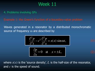
1. Week 11 4. Problems involving GFs Example 1: the Green’s function of a boundary-value problem Waves generated in a resonator by a distributed monochromatic source of frequency ω are described by (1) (2) where s(x) is the ‘source density’, L is the half-size of the resonator, and c is the speed of sound.

2. Physically, one should expect that, regardless of the initial condition, all of the wave field will sooner or later have the frequency of the source. Thus, let’s seek a solution of the form and Eqs. (1)-(2) yield (3) (4) Eqs. (3)-(4) are what we are going to work with (the preceding equations were included just to explain the problem’s physical background). It can be demonstrated that the solution to (3)-(4) is...

3. (5) Green’s function where G(x, x0) satisfies (6) (7) Physically, (6)-(7) describe the wave field from a point source of unit amplitude located at x = x0 – hence, solution (5) implies that we treat the original (distributed) source as a continuous distribution of point sources and just sum up (integrate) their contributions.

4. To prove the validity of solution (5)-(7), we shall substitute (7) into Eq. (3) and prove that its l.-h.s. and r.-h.s. are equal. As follows from (6), the [...] in the above equality is δ(x – x0) – hence, It is now evident that the l.-h.s. of (3) does equal its r.-h.s..

5. Before solving for G, we need to understand how the delta function affects it. To do so, integrate (6) from x0 – ε to x0 + ε, which yields (8) Next, multiply (6) by (x – x0) and repeat the same procedure again. Integrating the term involving G" by parts, we obtain (9)

6. Now, take the limit ε→0 and assume that G and G' remain finite (but not necessarily smooth or continuous) at x = x0. Then (8)-(9) yield hence, (10) (11) (11) tells us that the solution is continuous at x = x0, whereas (10) tells us that the solution’s derivative ‘jumps’ at x = x0.

7. (10)-(11) can be used as ‘matching conditions’ connecting the solution for x < x0 to that for x > x0. The delta function doesn’t contribute to either of these regions (as it’s ‘localised’ at x = x0), so we can forget about it. Essentially, it’s been replaced by (10)-(11). For x < x0, we have hence, (12) where k = ω/c, and A– is an arbitrary constant. Similarly, (13)

8. Use (10)-(11) to match (12) and (13) at x = x0: Solve these equations for A±: (14) where we have used the formula with a =x0 – Land b =x0 + L.

9. Summarising Eqs. (14)-(16), we obtain Observe that G(x, x0) is symmetric with respect to interchanging x and x0, which is usually the case with Green’s functions. This property is usually called the “mutuality principle”. Physically, it means that, if the wave source and the ‘measurer’ swap positions, the measurement doesn’t change.

10. Example 2: quantum particle in an infinitely narrow/deep well The 1D non-dimensional Schrödinger equation is (15) where ψ is the “wave function” (such that |ψ(x)|2is the probability of finding the particle at a point x), E is the particle’s energy, and u(x) is the potential of an external force. If, for example, the particle is an electron in an atom, u(x) would be the potential of the force of attraction exerted by the nucleus (and would have a minimum near that). We’ll be interested in bound states, for which (16) Those solutions that do not decay as x → 0 describe free particles.

11. Let Using the same trick as in the previous example, we can obtain ‘matching conditions’ connecting the x < 0 region to the x > 0 one: (17) (18) because of (18), it doesn’t matter whether it’s x = +0 or x = –0

12. Re-write the Schrödinger equation (15) in the form (we expect E to be negative (which corresponds to bound states) – hence, it’s convenient to use –E instead of E). The general solution of this equation is where A– and A+ are undetermined constants.

13. Imposing BC (16), we obtain Imposing the matching conditions (17)-(18), we obtain Solving for A± , one can see that a solution exists only if

14. Example 3: Fourier transform The forward and inverse Fourier transformations are usually defined by To prove that these are indeed inverse to each other, one needs to prove that hence...

15. (19) Observe that x is used in the inner integration, which was why we used x1 elsewhere (to avoid confusion). Change the order of integration in (19): (20) This equality holds only if (21)

16. Observe, however, that the integrand in (21) doesn’t decay as x → ±∞... so how do we evaluate this integral? This difficulty is due to the fact that, generally, the order of integration in a double integral can be changed only if this integral converges absolutely – but integral in (19) does not converge at all. So we shall use the following trick: consider the integral on the l.-h.s. of (19) as a limit of a family of slightly different integrals: For any ε > 0, the above integral is absolutely convergent – hence, we can change the order of integration and obtain...

17. (22) Evaluate the integral in []: hence...

18. (23) As proved in Problem 7.2, the above family of functions correspond to δ(x1 – x) – hence, (22) becomes which is clearly true. Thus, we have proved that the forward and inverse Fourier transformations are indeed inverse to one another.

19. Comments: • Physicists often use the formula which is a short-hand version of the statement that the family of functions (23) correspond to the delta function. • Physicists also use the formula which is a short-hand statement of the fact that...

20. and this family of functions corresponds to –πδ(x). The same result can be obtained from the Sokhotsky formula (Example 10.6).