Download
1 / 101
1.05k likes | 1.32k Vues
Overview of Regulatory 8-hr Ozone Modeling. T. W. Tesche Dennis McNally Alpine Geophysics, LLC Ft. Wright, KY Ralph Morris ENVIRON International Corp Novato, CA Farmington, NM 16 July 2003. Staff Credits Alpine Geophysics, LLC Dennis McNally Cyndi Loomis ENVIRON Int. Corp.

E N D
Overview of Regulatory 8-hr Ozone Modeling T. W. Tesche Dennis McNally Alpine Geophysics, LLC Ft. Wright, KY Ralph Morris ENVIRON International Corp Novato, CA Farmington, NM 16 July 2003
Staff Credits Alpine Geophysics, LLC Dennis McNally Cyndi Loomis ENVIRON Int. Corp. Ralph Morris
Workshop Topics • Role of Regulatory Photochemical Modeling in U.S. • Review of Ozone Photochemistry • Classification of Photochemical Models • Overview of the CAMx Regional Photochemical Model • Emissions Inventory Modeling • Meteorological Modeling • Model Performance Evaluation • Future Year Emissions Control Strategy Modeling • Ozone Attainment Demonstration
Ozone Concentration Trends for U.S. Cities: Los Angeles Ozone ppb 2nd Highest Value 4th Highest Value Year
Role of Regulatory Modeling • Areas that are not in compliance with the Federal National Ambient Ozone Standards (NAAQS) are required to use modeling to • Estimate the effects of growth (and expected control measures) on future ozone air quality • Evaluate alternative/additional measures • Demonstrate future compliance with 1-hr and 8-hr ozone standard(s) Regulatory modeling must follow prescribed EPA Guidance on model selection, episode selection, data base development, model performance evaluation, application of models, attainment demonstration, peer-review, and documentation
Role of Regulatory Modeling (concluded) • Modeling efforts for most areas include: • scoping study to assess the nature and extent of the problem and data gaps/needs • collection and analysis of meteorological, air quality, emissions, and land-use data • development and continued refinement of modeling databases and capabilities
Typical Regulatory Modeling Process Conceptual Model Development Select episodes and domains Prepare/refine inputs Model Evaluation Apply emiss, met, ozone models Compare model results to measurements No Performance OK? Yes Prepare future-year emissions Conduct future-year evaluations
Ozone Photochemistry • Sources and sinks for tropospheric ozone (“bad ozone”) • In contrast to stratospheric ozone (“good ozone”) • Ozone formation from VOC and NOx • Control strategy implications • Sensitivity to VOC and/or NOx • VOC reactivity • NOx suppression (inhibition or disbenefits) • Condensed chemical mechanisms
Sources and Sinks of Tropospheric Ozone • Sources • smog chemistry involving VOCs and NOx with sunlight • radical cycle among OH, HO2, RH2, etc. • global methane and CO oxidation • Stratospheric intrusion • Sinks • chemical reactions (e.g., NO, alkenes) • deposition
Ozone Formation from VOC and NOx no sunlight no ozone productionno NOx no ozone productionno VOC no ozone production
Control Strategy Implications ofVOC/NOx Chemistry • Sensitivity to emission reduction • VOC sensitive, NOx sensitive, or both • VOC reactivity • depends upon chemical nature: reaction rate, radical yields, products • approximated by reactivity scales, e.g., Carter MIRs • NOx suppression or inhibition • if ozone is highly VOC sensitive, NOx reduction may incur disbenefits • two mechanisms operative (1) direct titration (or scavenging) of ozone by fresh NO emissions (2) scavenging of radicals by NO2 inhibits ozone production
Ozone and Precursor Relationships: Ozone vs. NOz = reacted NOx (NO + NO2) • NOz = NOy - NOx • observed ozone/NOz relationship for a rural location in eastern U.S. • interpret slope as production efficiency for ozone from NOx (i.e., amount of ozone formed per NOx reacted away) NOz ppb
Key Photochemical Reactions NOx Reactions NO + O3 NO2 + O2 (NO-O3 titration) NO2 + NO + O (NO2 photolysis -- sunlight) O + O2 O3 (Ozone Formation) VOC-Radical Reactions VOC + OH VOC + HO2 (OH to HO2 w/o NO2 destruction) HO2 + NO OH + NO2 (NO to NO2 w/o O3 destruction) HO2 + HO2 H2O2 + O2 (H2O2 Formation) Secondary PM Reactions NO2 + OH HNO3 (Nitrate Formation -- Day) N2O5 + H2O HNO3 (Nitrate formation – Night) SO2 + OH SO4 + HO2 (Sulfate Formation – Gas-Phase) SO2 + H2O2 SO4 (Sulfate Formation – Aqueous) SO2 + O3 SO4 (Sulfate Formation – Aqueous) HNO3 (g) NO3 (pm) (Equilibrium – T, RH, NH3, SO4)
Classification of Photochemical Air Quality Simulation Models • Lagrangian employ a coordinate system that moves with air parcels • Eulerian the coordinate system is fixed in space • Hybrid incorporate features of Lagrangian types into a Eulerian framework
Photochemical Modeling Concepts All Air Models Solve Some Form of the Atmospheric Diffusion Equation (a complex differential equation) that Relates Changes in Pollutant Concentration to: • Advection (transport by the mean wind) • Turbulent diffusion • Chemical reaction • Deposition • Emissions
General Form of the SpeciesConservation (Continuity) Equation: Mathematical solution (integration) of general forms of the diffusion equation is difficult -- simplifying assumptions are required
Lagrangian Models • Many Simplifying Assumptions • Produce a simple, closed-form analytical expression for diffusion • Do not require numerical integration • Invoke the Assumption of Air Parcel Coherency • Breaks down quickly not far from an emissions source, especially in complex wind flow situations • Cost-effective solution at relatively close ranges for a relatively small number of sources
Lagrangian Models(continued) • Chemical interactions between puffs, segments, or particles cannot be properly treated • Readily produce source-receptor relationships • Severe technical limitations especially for: • large numbers of sources • regional-scale transport applications • photochemically reactive pollutants
Lagrangian Models(continued) Gaussian Plume Models • The earliest air models • Invoke many simplifying assumptions to obtain closed-form analytical solutions • Steady-state (i.e., time invariant) • Spatially uniform (homogeneous) dispersion • Plume coherency • Inert or first-order decay • Gaussian plume models are not capable of treating photochemistry
Lagrangian Models(continued) Examples of Gaussian Plume models include: • ISC • COMPLEX • RTDM • AERMOD
Lagrangian Models(continued) Gaussian Puff Models • Fewer simplifying assumptions • employ analytical solutions for each puff, but • computers are required to track the large number of puffs • still retain the plume coherency assumption • a few have been developed for individual reactive plumes, e.g., RPM-IV • numerical solution methods are needed to solve chemical kinetics equations
Lagrangian Models (continued) • Examples of Gaussian Puff models include: • CALPUFF • RPM-IV • SCIPUFF • SCICHEM
Processes Treated in a Grid Model • Emissions • Surface emitted sources (on-road and non-road mobile, area, low-level point, biogenic, fires) • Point sources (electrical generation, industrial, other, fires) • Advection (Transport) • Dispersion (Diffusion) • Chemical Transformation • VOC and NOx chemistry, radical cycle • [For PM aerosol thermodynamics and aqueous-phase chemistry] • Deposition • Dry deposition (gas and particles) • Wet deposition (rain out and wash out, gas and particles)
Eulerian Models • Generally considered to be technically superior • allow more comprehensive, explicit treatment of physical processes • chemical processes included • interactions of numerous sources • Require sophisticated solution methods • employ discrete time steps and operator splitting • computational grid (hence the term “grid models”) • relatively expensive to apply for long periods
Eulerian Models (continued) • Subgrid resolution can be a limitation • as grid size and time step length are reduced • accuracy increases, but • computation time also increases • advanced grid models employ variable grid spacing or nesting • improves accuracy in critical locations • allows cost effective application on urban to regional scales • CAMx has flexi-nesting capability
Hybrid (Lagrangian/Eulerian) Models • Incorporate features of Lagrangian models into grid model framework • overcome many of the sub-grid model limitations • Overcome many of the prior practical advantages of Lagrangian models, through the development of: • variable (nested) grid resolution • source apportionment techniques • Capitalize on the availability of low-cost high speed computers
Hybrid Models (concluded) • Examples of hybrid photochemical grid models include: • MODELS-3/CMAQ • MAQSIP • UAM-V • CAMx
Modules in a Grid Model • Emissions Modeling System • EPS2x, SMOKE and EMS-2003 • Meteorological Modeling System • MM5 and RAMS (SAIMM and CALMET) • Preprocessors for Other Inputs • TUV (photolysis Rates) • Initial Concentrations and Boundary Conditions • Air Quality Model • CAMx/PMCAMx, Models-3/CMAQ (UAM-V, MAQSIP) • Post-Processors and Visualization • Model Performance Evaluation (MAPS, CAMXtrct, Excel, SURFER) • PAVE • Flying Data Grabber
General Model Summary Photochemical grid/hybrid models have evolved as the preferred means of addressing complex and nonlinear processes affecting reactive air pollutants in the troposphere These models invoke fewer assumptions but require high speed computers and sophisticated numerical integration methods Higher accuracies require more computer resources Modern hybrid models utilize variable grid spacing (nested grids) in combination with a Lagrangian puff sub-model to treat subgrid resolution of plume dispersion and chemistry
Overview of the CAMx Regional Photochemical Model • Simulates the physical and chemical processes governing the formation and transport of ozone in the troposphere • three-dimensional, Eulerian (grid-based) model • requires specification of meteorological, emissions, land-use, and other geographic inputs • output includes hourly concentrations of ozone and precursor pollutants for each grid cell within a (three-dimensional) modeling domain
CAMx Overview (continued) Mathematically simulates the following processes: • emission of ozone precursors (anthropogenic and biogenic) • advection and diffusion (transport) • photochemistry • deposition
Example of a Multiply Nested CAMx Domain: Denver 8-hr EAC Study 4-km grid 36-km grid 12-km grid 1.3-km grid
CAMx Model Formulation Change in Concentration = Advection by Winds Turbulent Diffusion + Ri + Si + Li Emissions Surface Removal/Deposition Chemical Reaction
CAMx Modeling System Features • Carbon-Bond-IV chemical mechanism with enhanced isoprene and toxics chemistry • Two-way interactive nested-grid capabilities • Plume-in-grid (P-i-G) treatment • Accepts output from a variety of dynamic meteorological models
CAMx Input Requirements • Meteorological Inputs • Three-dimensional winds • Three-dimensional temperatures • Three-dimensional water-vapor concentration • Surface pressure • Three-dimensional vertical diffusivity (effective mixing height) • Two-dimensional cover • Rainfall rate
CAMx Inputs (continued) • Emissions Inputs • Low-level anthropogenic emissions • Point sources • Area sources • On-road motor vehicles • Non-road sources • Elevated point source emissions • Biogenic emission estimates
CAMx Inputs (continued) • Air quality related input files • Initial conditions (all grids, initial hour) • Boundary conditions (outermost grid, all hours) • Chemistry input files • Chemical reaction rates • Photolysis rates • Geographic/other input files • Land-use, Land-cover • Albedo, turbidity, and ozone column
CAMx Probing Tools • “Probing Tool” • A module within the photochemical grid model that extracts information on source-receptor relationships, chemical and physical processes, mass flux, etc. • Used to diagnose model to understand why it is getting the answer it gets and improve modeling performance • Used to better define optimal emission control strategies
Probing Tools in CAMx • Decoupled Direct Method (DDM) – first-order sensitivity coefficients of ozone by emission source groups (also in URM and CMAQ models) • Ozone Source Apportionment Technology (OSAT) – ozone source apportionment by source groups (source category + geographic region) • Process Analysis – output information on chemical processes and mass flux (also in CMAQ)