Download
1 / 34
340 likes | 413 Vues
Learn about speedup, efficiency, load imbalance, overhead, Amdahl’s Law, granularity, and scalability in parallel performance. Understand the impact of processor allocation on performance metrics like speedup and efficiency.

E N D
Lesson 8 ParallelPerformance Measurement Dr. Stephen Tse stephen_tse@qc.edu
Speed Up 1. Speed Up Let T(1, N) be the time required for the best serial algorithm to solve problem of size N on 1 processor and T(P, N) be the time for a given parallel algorithm to solve the same problem of the same size N on P processors. Speedup is defined as S(P, N) = T(1,N)/T(P, N) Remarks: • Normally, S(P,N) < P; Ideally, S(P,N) = P; Rarely, S(P,N) > P --- super speedup. • Linear speedup: S(P,N) = c*P where c is a constant independent of N and P. • Algorithms with S(P,N) = c P are called scalable algorithm.
Parallel Efficiency 2. Parallel Efficiency Let T(1, N) be the time required for the best serial algorithm to solve problem of size N on 1 processor and T(P, N) be the time for a given parallel algorithm to solve the same problem of the same size N on P processors. Parallel efficiency is defined as E(P,N)= T(1, N)/[T(P, N)P] = S(P,N)/P Remarks: • Normally, E(P,N) < 1; Ideally, E(P,N) = 1; Rarely, E(P,N) > 1; E(P,N) ~.6 acceptable. Of course, it is problem-dependent. • Linear speedup: E(P,N) = c where c is a constant independent of N and P. • Algorithms with E(P,N) = c are called scalable algorithms.
3. Load Imbalance Ratio I(P,N) • Processor i spends ti doing useful work and tmax = max{ti} is the maximum time spent by one or more processors and tavg= (i=0P-1 ti)/P= average time The total time spent on useful task for computation and communication is i=0P-1 ti while the time that the system is occupied (either computation or communication or idle) is P tmax. Thus, we define a parameter called load imbalance ratio: I(P,N) = [Ptmax - i=0P-1 ti]/ i=0P-1 ti = tmax / tavg – 1 Remarks: 1. Per processor wasted time= tavg * I(P,N) = tmax-tavg • I(P,N) is the average time wasted by each processor due to load imbalance. • If tmax =tavg, then ti = tavg, then, I(P,N) = 0 this implies complete load balance. • One slow (not doing what it suppose to do) processor (tmax) can mess up the entire team. This observation shows that Slave-Master scheme is usually very inefficient because of the load imbalance issue due to slow master processor. Therefore, Slave-Master scheme is usually avoided.
Overhead 4. Overhead • A parameter h(P,N) is defined by E(P,N)= 1/[1 + h(P,N)] where h(P,N) is called overhead and it can be solved as 1 P h(P,N) = - 1 = - 1 E(P,N) S(P,N) • Remarks: • h(P,N) measures time spent result from communication and load imbalance. • h(P,N) if E(P,N) 0. • h(P,N) 0 if E(P,N) 1.
Amdahl’s Law 5. Amdahl’s Law Suppose a fraction of an algorithm for a problem of size N on P processors is inherently serial and the remainder is perfectly parallel, then assume T(1,N) = . Thus, T(P,N) = f + (1-f) /P Therefore, S(P,N) =1/[f + (1-f)/P] This equation indicates that when P, the speedup S(P,N) is bounded by 1/f. It means that the maximum possible speedup is finite even if P.
Granularity 6. Granularity The size of the problem allocated to individual processors is called the granularity of the decomposition. Remarks: • Granularity is usually determined by the problem size N and computer size P. • Decreasing granularity usually increases communication and decreases load imbalance. • Increasing granularity usually decreases communication and increases load imbalance.
Total Overhead Overhead
Scalability • Ascalable algorithm is that whose E(P, N) remains bounded from below, i.e., E(P, N) E0 > 0, when the number of processors P at fixed problem size. A quasi-scalable algorithm is that whose E(P, N) remains bounded from below, i.e., E(P, N) E0 > 0, when the number of processors Pmin < P < Pmax at fixed problem size. The interval [Pmin, Pmax] is called scaling zone. Remarks: • True scalable: rare; quasi-scalable: often. • Quasi-scalable is usually regarded as scalable. • At fixed N=N(P), E(P,N(P)) decreases monotonically as P increases. But, this relationship is problem-dependent. • At fixed P=P(N), E(P(N), N) increases monotonically as N increases. But, this relationship is problem-dependent. • Efforts: maximize scaling zone [Pmin, Pmax] and E0.
Principles: minimizing overhead. • Principles: minimizing overhead. • Minimize communication-to-computation ratio. • Minimize load imbalance • Maximize scaling zone
Lesson 8-a C Programming Dr. Stephen Tse stse@forbin.qc.edu 908-872-2108
C Language • C is a general purpose programming language • C provides variety of data type: • characters, integers, and floating-point numbers. • Derived data types created with pointers, arrays, structures, and unions • Expression: formed from operators and operands; • Pointers: provide for machine-independent address arithmetic.
C Control-flow • statement grouping, decision making (if-else) • selecting one of a set of possible cases (switch) • looping with the termination test at the top (while, for) • looping with the termination test at the bottom (do) • early loop exit (break)
C Functions • Functions may return values of basic types, structures, unions, or pointers. • Any function may be called recursively. • Function definitions may not be nested but variables may be declared in a block-structured fashion. • Variables may be internal to a function, external but known only within a single source file, or visible to the entire program.
Getting Started • The first program to print ‘hello world” #include <stdio.h> /*Include info of standard lib*/ main() /*Define a function - Main*/ { /* statements are enclosed in braces */ printf(“hello, world\n”); /* calls the print function */ } /* \n is a new line character */ The first C program • You must create the program in a file whose name ends in “.c”, then compile it with the command: cc hello.c • If the program has no error, the compilation will be silent and creates an executable file called a.out • If you run the a.out by typing this command; it will print hello, world
Anatomy of a C program • C program consists of functions and variables. • A function contains statements that specify the computing operations. to be done. • Variables store values used during the computation. • Every C program has a “main” and the program begins execution at the beginning of main.
main () • “main” calls other functions to help perform its job; some that you wrote, and others from libraries that are provided for you. • Therefore, the first line of the program is always include the standard input/output library: #include <stdio.h>
arguments • f(arg1, arg2) - communicating data between functions is for the calling function to provide a list of values, called arguments, to the function it calls. The parentheses after the function name surround the argument list. Functions have no arguments are represented by the empty list ().
Variables and Arithmetic Expressions • All variables must be declared before they are used. A declaration announced the property of the variables: • lnt (integer) fahr, celsius; • char (character-a single byte) • short (short integer) • double (double-precision floating point) • float (floating point, numbers represented by decimal) • If Arithmetic Expressions has one floating point operand, all integers will be converted to float before opration.
Pointers and Arrays • A pointer is a variable that contains the address of the variable: int *P ; /* P is a pointer */ P = &C ; /* P now point to C */ C: P: 201 203 . . . . 875 874 875 . . . . 874 3.1416 Add. of C Content int x=1, y=2, z[10]; int *iP; iP=&x; /* iP now points to x */ y=*iP; /* Unary operator * applied to a pointer, it access the object the pointer points to. So, y now is 1 */ *iP=0; /* x now is 0 */ ip=&z[0]; /* iP now point to the beginning of array z[0] */ What are the following: y=*ip+1; /* y = whatever iP points to add 1. */ *ip += 1; /* Increments what ip points to */ or ++*ip; or (*ip)++;
swap(a,b) • C passes arguments to functions by value, there is no direct way for the called function to alter a variable in the calling function. • It is not enough to write: swap(a, b); where the swap is: void swap(int x, int y) /* WRONG */ { int temp; temp = x; x = y; y = temp; } Instead: void swap(int *px, int *py) /* interchange *px and * py */ { int temp; temp = *px; *px = *py; *py = temp; }
printf and format • printf(“%3.0f %6.f\n”, fahr, celsius) • “ … “ is the character string to be printed. • variable can have different data type: • char a single byte, capable of holding one character (8 bits) • int an integer (either 16 or 32 bits) • short short interger, (16 bits) • long long integer (32 bits) • float single-precision floating point (contain a decimal point or an exponent) • double double-precision floating point • print as: • %d print as decimal integer • %6d print as decimal integer, at least 6 characters wide • %f print as floating point • %.2f print as floating point, 2 character after decimal point • %6.2f print as floating point, at least 6 character wide and 2 after decimal point. • %s print as character string • %o print octal • %x print hexadecimal • %c print as character
Data-object type categories TYPE CATEGORIES char int enum float double _segment Pointers Arrays Structures Unions Integral Floating-Point Aggregate arithmetic scalar
Constants • Integer constant: 1234 is an int. • A long constant: 123456789L is written with a terminal l (ell) or L. • Unsigned constant: is written with a terminal u or U. the suffix of ul or UL indicates unsigned long. • Floating-point constant: contains a decimal point (123.4) or an exponent (1e-2) or both; their type is double. The suffix f or F indicate a float constant; l or L indicate a long double. • Octal: a leading 0 (zero) on an integer constant • Hexadecimal: a leading 0X or 0x means hexadecimal. • Character constant: is an integer, written as one character within single quotes, such as ‘0’ (zero); has the value 48, which is unrelated to the numeric value 0. • Escape sequences: certain characters can be represented in string constants by escape sequences like \n (newline) which looks like two characters, but represent only one. • \000 one or three octal digits (0…7) • \xhh where hh is one or more hexadecimal digits (0…9,a…,f, A…F) • \013 for vertical tab • \007 for bell character • \a Alert (bell) character \\ backslash • \b backspace \? question mark • \f formfee \’ single quote • \n newline \” double quote • \r carriage return \0 null character, end of string with value 0 • \t horizontal tab EOF end of file • \v vertical tab
Function and if statement • A function definition has this form: return-type function-name(parameter declarations, if any) { declarations statements } • The if logical pattern if ( condition1) statements1 else if (condition2) statements2 … … … … else statementn Remark: if every conditions fail, the final statement will be executed True False out False True out False out Final
String Termination • A string constant: “hello\n” • It is stored as an array of characters containing the characters of the string and terminated with a ‘\0’ to mark the end. h e l l o \n \0 Remark: The ‘\0’ is not a part of the normal text; but the %s string format expects the input argument is terminated by ‘\0’, and it copies this character into the output argument.
Type Conversion • When an operator has operands of different types, the “narrow” operand is automatically converted to the “wider” one. • If either operand is long double, convert the other to long double. • Otherwise, if either operand is double, convert the other to double. • Otherwise, if either operand is float, convert the other to float. • Otherwise, convert char and short to int. • Then, it either operand is long, convert the other to long. • Finally, explicit type conversions can be forced (“coerced”) in any expression with a unary operator called a cast. (type name) expression the expression is converted to the named type.
Random Numbers • Many simulations do not simulate events given by input data, but rather generate events according to some probability distribution. A random number generating function rand(x) is used. • The starting point of the pseudorandom integer, x, called the seed, is set by calling srand(x). The default seed for rand is 1. The same seed will generate the same set of random sequence for rand. • the statement x=rand(x) resets the value of the variable x to a uniform random real number between 0 and Rand_Max(32767). • The following statements (where a and b are integers): x=rand(x); y=(b-a)*x+a The variable y is said to be a uniformly distributed random variable between a and b-1. a b 0 32,767 y x Result = Low + (High – Low)*number Pseudo-random numbers: srand ((unsigned) Time(NULL)); use Time as a seed to generate integers between 0 and 32,767 (RAND_MAX)
Algorithms to Generate Pseudorandom Numbers – Linear Congruential Algorithms • Developed by D.H. Lehmer around 1950, to use the four integer parameters to generate a pseudorandom sequence: • The starting (or current/seed) value, X0(or Xn) • The multiplier, a (greater than or equal to 0) • The incrementer, c (greater than or equal to 0) • The modulus, m (must be the largest & greater then 0) • The formula: Xn+1 = (aXn + c) % m (% is the modular operator.) The formula will generate random value between 0 and m-1, inclusive. If m=10, the formula will generate random values between 0 and 9, inclusive. If the modulus parameter chose to be close to the maximum possible signedint (32767). The formula will produce good random numbers.
Assignment Operations • The operator += is called an assignment operator. • Most binary operators have a left and a right operand with a corresponding assignment operator “op=“, where op is one of: + - * / % << >> & ^ | • If expr1 and expr2 are expressions, then expr1 op= expr2 is equal to expr1 = (expr1) op (expr2) • For example: expr1 /= expr2 is equal to: expr1 = expr1 expr2
Conditional Expressions • The conditional expression, written with the ternary operator “?:”, provides an alternate way to write: it (a>b) z = a; else z = b; • The similar construction in conditional expression: expr1? expr2: expr3 The expr1 is evaluated first. If it is non-zero (true), then the expr2 is evaluated and that is the value of the conditional expression. Otherwise exp3 is evaluated, and that is the value.