Autocorrelation II
Autocorrelation II. Lecture 21. Today’s plan. Durbin’s h-statistic Finite Distributed Lags Koyck Transformations and Adaptive Expectations Seasonality Testing in the presence of higher order serially correlated forms. 0. 2. 4. d = 0.331. 1.475. d L. 4-d U. 4-d L. d U. H 0 : = 0.


Autocorrelation II
E N D
Presentation Transcript
Autocorrelation II Lecture 21
Today’s plan • Durbin’s h-statistic • Finite Distributed Lags • Koyck Transformations and Adaptive Expectations • Seasonality • Testing in the presence of higher order serially correlated forms.
0 2 4 d = 0.331 1.475 dL 4-dU 4-dL dU H0: =0 H1 H1 Reject null Reject null Accept null Returning to the Durbin-Watson • Last time we talked about how to test for autocorrelation using the Durbin-Watson test • We found autocorrelation in the data in L_20.xls • We used this figure:
Generalized least squares (3) • Need an estimate of : we can transform the variables such that: where: • Known as Cochrane-Orcutt transformation. • Estimating equation (3) allows us to estimate in the presence of first-order autocorrelation
Problems 1) The model presented by may still have some autocorrelation • the D-W test doesn’t tell us anything about this • we have to retest the model 2) We may lose information when we lag our variables • to get around this information loss, we can use the Prais-Winsten formula to transform the model:
Problems (2) 3) We might want to include a lagged endogenous variable in the model • including the lagged endogenous variable Yt-1 biases the Durbin-Watson test towards 2 • this means it’s biased towards the null of no autocorrelation • in this instance, we’ll use Durbin’s h-statistic (1970): v = square of the standard error on the coefficient (g) of the lagged endogenous variable
Durbin’s h-statistic • Durbin’s h-statistic is normally distributed and is approximated by the z-statistic (standard normal) • null hypothesis: H0: = 0 • the null can be rejected at the 5% level of significance • L21.xls has example. • Problems with the h-statistic • the product nv must be less than one (where n = # of observations) • if nv 1, the h-statistic is undefined
A note on consistency • Model with lagged endogenous variable and first-order serially correlated error may be mis-specified. Yt = b0 + b1Yt-1 + ut and ut = rut-1 + et • If so, presence of first-order serial correlation may induce omitted variable bias. • Need to include additional lagged endogenous variable term: Yt = a0 + a1Yt-1 + a2Yt-2 + et
Why lags? • This mainly relates to macroeconomic models • economic events such as consumer expenditure, production, or investment • for instance: consumer expenditure this year may be related to consumer expenditure last year • In a general distributed lag model: Yt = a + b0Xt + b1Xt-1 +…+bkXt-k + et • where k = any large number less than t-2 • can eliminate coefficients b1 to bk by using a t-test • number of lags included is ad-hoc
Problems for OLS • Lags lead to severe problems for ordinary least squares • loss of information (degrees of freedom) • independent variables (X) are highly correlated [multi-collinearity problem]
Why lags are useful • Psychological reasons: behavior is habit-forming • so things like labor market behavior and patterns of money holding can be captured using lags • Technological reasons: a firm’s production pattern • Institutional: unions • Multipliers: short run and long run multipliers (how to read finite distributed lags in a model).
Ad-hoc nature of lags • What can we do? • Two approaches • Koyck transformation • Adaptive expectations • Different implications on the assumptions about economic processes • will end up with the same estimating equation • looking only at the end product, we won’t be able to tell the Koyck transformation from adaptive expectations
Koyck transformation • Model: Yt = a + b0Xt + b1Xt-1 +…+bkXt-k + et • The Koyck transformation suggests that the further back in time we go, the less important is that factor • for instance, information from 10 years ago vs. information from last year • The transformation suggests: Where 0 < < 1 j = 1,…k
Koyck transformation (2) • So, • Can use the expression for bj to rewrite the model Yt = a + b0 (Xt + Xt-1 + 2Xt-2 + ….+ kXt-k) + et(4) • this imposes the assumption that earlier information is relatively less important • Lagging the equation and multiplying it by , we get: Yt-1 = a + b0 (Xt-1 + 2Xt-2 + ….+ kXt-k) + et-1 (5) • Subtracting (5) from (4), we get Yt = a(1- ) + b0Xt + Yt-1 + vt where vt = et - et-1
Koyck transformation (3) • Why is this transformation useful? • Allows us to take the ad-hoc lag series and condense it into a lagged endogenous variable • now we only lose one observation due to the lagged endogenous variable • the given by the estimation gives the coefficient of autocorrelation • Problem: by construction, we have first-order autocorrelation • use Durbin h-statistic • but estimating equation might be mis-specified!
Adaptive expectations • Another way to approach the problem of the ad-hoc nature of lags • Can use the example of trying to measure the natural rate of unemployment • In 1968, Friedman estimated the equation: Yt = a + bXt* + ut where Xt* = natural rate of unemployment
Adaptive expectations (2) • Using adaptive expectations we have that Xt* - Xt-1* = (Xt - Xt-1*) • Can rewrite the equation: Xt* - (1 - )Xt-1* = Xt • Using a lag operator where: LXt = Xt-1 L2Xt = Xt-2 where Xt* = expectation Xt = observed 0 < < 1
Adaptive expectations (3) • We can then rewrite : Xt = (1 - L )Xt* • where = (1- ) • This can be rewritten as: • now we have the natural rate of unemployment in terms of the observed rate of unemployment
Adaptive expectations (3) • Substituting into the model we get: • Upon further multiplication and substitution we arrive at: • this looks very similar to that for the Koyck transformation where
Problems with the approaches • For the lagged endogenous variables in the ad-hoc lag structure, we are uncertain as to which economic model of agent behavior underlies the estimating equation • We have 1st-order autocorrelation by the construction of the model • use the Durbin h-statistic • Yt-1 and et-1 (ut-1) are sure to be correlated [ E(X,e) 0] • this leads to biased estimates • we’ll deal with this using instrumental variables and simultaneous equations
Other topics • Seasonality and the use of dummy variables in time series models. • Trends and their use in time series models • Testing and correcting in the presence of higher orders of serial correlation.