Download
1 / 32
320 likes | 447 Vues
This final year project outlines an innovative system for video object tracking and replacement, enhancing post-TV production capabilities. It discusses the essential components, including bitmap readers, RGB to HSV conversion, edge detection, and texture mapping, which collectively allow for sophisticated object manipulation. The system aims to reduce production costs, facilitate dangerous scene edits, and create effects unattainable in reality. Future work will focus on optimizing algorithms for real-time applications, addressing current challenges in object detection, and expanding the system's functionality.

E N D
Video Object Tracking and Replacement for Post TV Production LYU0303 Final Year Project Fall 2003
Outline • Project Introduction • Basic parts of the purposed system • Working principles of individual parts • Future Work • Q&A
Introduction • Post-TV production software changes the content of the original video clips. • Extensively used in video-making industries. • Why changing the content of a video? • Reducing video production cost • Performing dangerous actions • Producing effects those are impossible in reality
Difficulties to be overcome • Things in video can be treated individually called “video objects”. • Computers cannot perform object detection directly because… • Image is processed byte-by-byte • Without pre-knowledge about the video objects to be detected • Result is definite, no fuzzy logic. • Though computers cannot perform object detection directly, it can be programmed to work indirectly.
Basic parts of the purposed system • Simple bitmap reader/writer • RGB/HSV converter • Edge detector • Edge equation finder • Equation processor • Translation detector • Texture mapper
RGB/HSV converter • Human eyes are more sensitive to the brightness rather than the true color components of an object. • More reasonable to convert the representation of colors into HSV (Hue, Saturation and Value (brightness)) model. • After processing, convert back to RGB and save to disk.
RGB to HSV HSV to RGB RGB/HSV converter
Edge detector • Usually, a sharp change in hue, saturation or brightness means that there exist a boundary line. HSV: (0,0,0) HSV: (0,255,255)
Edge equation finder • Derives mathematical facts out of the edge points. • Works with voting algorithm of Hough Transform. • Automatically adjusts tolerance value to minimize the effect of noise points. • This helps when the edge is not completely straight or blurred.
Edge equation finder Angle in degree Frequency 0 1 45 3 90 1 135 1 (x1,y1) Desired linear equation in point-slope form:
Equation processor • After finding out the equation, constraints can be applied in order to remove redundant equations, get shadows or detect occultation. • Find out the corner points for translation detector and texture mapper.
Translation detector • A simple object motion tracker. • Collects the data of the first key frame to accelerate the process of the remaining video frames. • Can be beneficial if the video segment is long and the scene seldom changes.
Texture Mapper • A graphics design process in which a 2-D surface, called a texture map, is "wrapped around" a 3-D object. • The 3-D object acquires a surface texture similar to the texture map.
Texture Mapper Mapping New position of pixel Original position of pixel
Texture Mapper • Every polygon is assigned 2 sets of coordinates • Image coordinates (r, c): location of pixel in the image • Texture coordinates (u, v): location in texture image which contains color information for image coordinates
Texture Mapper • Mapping functionsmap texture coordinates to image coordinates or vice versa. • They are usually determined by image points whose texture coordinates are given explicitly.
Texture Mapper (u1, v1) (u2, v2) (r1, c1) (u1, v1) (r2, c2) (u2, v2) (r4, c4) (u4, v4) (r3, c3) (u3, v3) (u4, v4) (u3, v3)
Texture Mapper • Scan conversion: the process of scanning all the pixels and perform the necessary calculation. • Forward mapping maps from the texture space to image space • Inverse mapping maps from the image space to texture space
Scan conversion with forward mapping • Algorithm: • for u = umin to umax • for v = vmin to vmix • r = R(u,v) • c = C(u,v) • copy pixel at source (u,v) • to destination (r,c)
Scan conversion with forward mapping • Advantage: Easy to compute as long as the forward mapping function is known. • Disadvantage Pixel-to-pixel mapping is not 1-1. Holes may appear. Can result in aliasing.
Scan conversion with inverse mapping • Algorithm: • for (r,c) = polygon pixel • u = TEXR(r,c) • v = TEXC(r,c) • copy pixel at source (u,v) • to destination (r,c)
Scan conversion with inverse mapping • Advantage: Every destination pixel is filled (no holes). Allow easy incorporation of pre-filtering & resampling operations to prevent aliasing
Scan conversion with inverse mapping • Take advantage of Scanline Polygon Fill Algorithm • For a row scan, maintain a list of scanline / polygon intersections. • Intersection at scanline r+1 efficiently computed from row r. {xk+1, yk+1} Scanline yk+1 Scanline yk {xk, yk}
Scan conversion with inverse mapping • Coordinates at a non-boundary level are computed by linearly interpolating (u,v) coordinates of bounding pixels on the scanline. {xk+1, yk+1} Scanline yk+1 Scanline yk {xk, yk}
Scan conversion with inverse mapping • Suppose (ri,ci) maps to (ui,vi), i = 1,…, 5 • (r4,c4) = s (r1,c1) + (1-s) (r3,c3) { s is known } • (u4,v4) = s(u1,v1) + (1-s)(u3,v3) {u4,v4 are known} • Similarly, (u5, v5) can be found. • t = (c-c4)/(c5-c4) • (r,c) = t*(u5,v5) + (1-t)*(u4,v4) (r1, c1) (r, c) Scanline yk (r4, c4) (r5, c5) image (r3, c3) (r2, c2)
Basic 2D linear mapping • Scaling & Translation u = ar + d v = bc + e upright rectangle upright square • Euclidean mapping u = (cos)r – (sin)c + d v = (sin)r + (cos)c + e rotated unit square upright square
Basic 2D linear mapping • Similarity mapping u = s(cos)r – s(sin)c + d v = s(sin)r + s(cos)c + e rotated square upright unit square • Affine mapping u = f(cos)r – g(sin)c + d v = h(sin)r + i(cos)c + e rotated rectangle upright unit square DEMO !
Basic 2D linear mapping • Projective mapping The most general 2D linear map Square arbitrary quadrangle ! • u = (a11r+a12c+a13) / (a31r+a32c+1) • v = (a21r+a22c+a23) / (a31r+a32c+1) • The 8 variables a11,a12, … , a32 have to be found out.
Basic 2D linear mapping • We have a system of 8 equations solving 8 unknowns. (x1,y1)
Future Work • Mapping cans • Speed optimization • Movie manipulation • Use of 3D markers
Q & A See the foot notes.