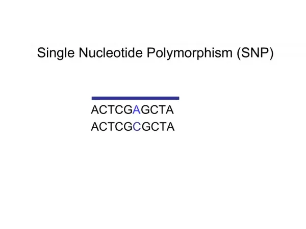
Single Nucleotide Polymorphism
Single Nucleotide Polymorphism. Some people have blue eyes, some are great artists or athletes, and others are afflicted with a major disease before they are old.

Single Nucleotide Polymorphism
E N D
Presentation Transcript
Single Nucleotide Polymorphism Some people have blue eyes, some are great artists or athletes, and others are afflicted with a major disease before they are old. Many of these kinds of differences among people have a genetic basis - alterations in the DNA. Sometimes the alterations involve a single base pair and are shared by many people. Such single base pair differences are called "single nucleotide polymorphisms", or SNPs for short. Nonetheless many SNPs, perhaps the majority, do not produce physical changes in people with affected DNA. (On average, SNPs occur in the human population more than 1 % of the time. Since only 3-5% of the genome code for proteins, most SNPs are found outside of coding regions. Those within a coding region are of course of particular interest.) Why then are genetic scientists eager to identify as many SNPs as they can, distributed on all 23 human chromosomes? Bioinformatics III
Reasons for studying SNPs 1 Even SNPs that do not themselves change protein expression and cause disease may be close on the chromosome to deleterious mutations. Because of this proximity, SNPs may be shared among groups of people with harmful but unknown mutations and serve as markers for them. Such markers help unearth the mutations and accelerate efforts to find therapeutic drugs. 2 Analyzing shifts in SNPs among different groups of people will help population geneticists to trace the evolution of the human race down through the millenia and to unravel the connections between widely dispersed ethnic groups and races. 3 Most human sequence variation is attributable to SNPs, with the rest attributable to insertions or deletions of one or more bases, repeat length polymorphisms and rearrangements. Bioinformatics III
The SNP Consortium These motives motivated a number of pharmaceutical and technology companies and academic sequencing centers to join forces to identify thousands of SNPs. - The task is smaller than sequencing the whole human genome - 4 major centers for genetics involved: Cold Spring Harbor Lab, Sanger Centre, Wash Univ St. Louis, Whitehead/MIT Center for Genome Research The fruits of this research are made available in the database dbSNP: www.ncbi.nlm.nih.gov/SNP/ Main publication: A map of human genome sequence variation containing 1.42 million SNPs, The international SNP Map Working Group (41 authors) Nature 409, 928 (2001). In this work, single base differences were detected using two validated algorithms: Polybayes and the neighbourhood quality standard (NQS). Bioinformatics III
POLYBAYES Develop + test with EST clones from 10 genomic clones that are aligned against a fragment of the finished sequence of human (less than 1 error per 10.000 bp). Task is to identify SNPs from the genomic sequences of multiple individuals (e.g. 10 genomic clones). First organize sequences: - fragment clustering - identification of paralogues (induction of sequences representing highly similar regions duplicated elsewhere in the genome may give rise to false SNP predictions) - multiple alignment of sequences - analyze differences among sequences (e.g. using Polybayes) Marth et al. Nature Gen. 23, 452 (1999) Bioinformatics III
Application of the POLYBAYES procedure to EST data Regions of known human repeats in a genomic sequence are masked. b, Matching human ESTs are retrieved from dbEST and traces are re-called. c, Paralogous ESTs are identified and discarded. d, Alignments of native EST reads are screened for candidate variable sites. e, An STS is designed for the verification of a candidate SNP. f, The uniqueness of the genomic location is determined by sequencing the STS in CHM1 (homozygous DNA). g, The presence of a SNP is analysed by sequencing the STS from pooled DNA samples. Marth et al. Nature Gen. 23, 452 (1999) Bioinformatics III
Paralogue identification Identify paralogous sequences by determining if the number of mismatches observed between the genomic reference sequence and a matching EST is consistent with polymorphic variation opposed to sequence difference between duplicated chromosomal locations, taking into account sequence quality. Observation: paralogous sequences exhibit a pair-wise dissimilarity rate higher than PPAR= 0.02 (2%) compared with the average pair-wise polymorphism rate, PPOLY,2 = 0.001 (0.1%) In a pair-wise match of length L we therefore expect L PPOLY,2 mismatches due to polymorphism, versus L PPAR mismatches due to paralogous difference. In both cases, an additional number, E, of mismatches are expected to arise from sequencing errors. Expect DNAT = L PPOLY,+ E or DPAR = L PPAR+ E mismatches. Marth et al. Nature Gen. 23, 452 (1999) Bioinformatics III
Paralogue identification The probability of observing d discrepancies in the pairwise alignment is approximated by a Poisson distribution, with parameter = DNAT for ModelNAT and = DPAR for ModelPAR. In the absence of reliable a priori knowledge of the expected proportions of native versus paralogous ESTs, uninformed (flat) priors were used. The posterior probability PNAT = P(ModelNAT|d) that the EST represents native sequence is estimated as: ESTs that scored above a cutoff value, PNAT,MIN, were considered native; sequences scoring below the threshold were declared paralogous. Marth et al. Nature Gen. 23, 452 (1999) Bioinformatics III
Paralogue discrimination Example probability distributions for a matching sequence with (hypothetical) uniform base quality values of 20, in pair-wise alignment with base perfect genomic anchor sequence (quality values 40), over a length of 250 bp. PPOLY,2 = 0.001, PPAR = 0.02, E = 2.525, DNAT= 2.775 and DPAR = 7.525. Note: the error rate E is quite similar to the frequency of true polymorphisms DNAT ! If the posterior probability, PNAT, is higher than PNAT,MIN, the EST is considered native; otherwise, it is considered paralogous. Marth et al. Nature Gen. 23, 452 (1999) Bioinformatics III
Paralogue discrimination Distribution of the posterior probability values, PNAT, calculated for 1,954 cluster members from real EST data anchored to ten genomic clone sequences. The bimodal distribution indicates that one can distinguish between less accurate sequences that nevertheless originate from the same underlying genomic location, and more accurate sequences with high-quality discrepancies that are likely to be paralogous. Using PNAT,MIN = 0.75, 23% of the cluster members were declared as paralogous. Marth et al. Nature Gen. 23, 452 (1999) Bioinformatics III
SNP detection The Polybayes algorithm identifies polymorphic locations by evaluating the likelihood of nucleotide heterogeneity within (perpendicular) cross-sections of a multiple alignment = single nucleotide positions. Each of the nucleotides S1, ..., SN, in a cross-section of N sequences, R1, ..., RN, can be any of the four DNA bases, for a total of 4N nucleotide permutations. The likelihood P(Si|Ri) that a nucleotide Siis A, C, G, or T is estimated from the error probability PError,i obtained from the base quality value. (1 - PError,i) is assigned to the called base, and (PError,i/3) to each of the three uncalled bases. In the absence of likelihood estimates, insertions and deletions are not considered. Marth et al. Nature Gen. 23, 452 (1999) Bioinformatics III
SNP detection in multiple alignments Each heterogenous (polymorphic) permutation is classified according to its nucleotide multiplicity, the specific variation, and the distribution of alleles. The value PPOLY = 0.003 (1 polymorphic site in 333 bp) was used as the total a priori probability that a site is polymorphic. The values PPoly have to be distributed to assign a prior probability PPrior(S1, ..., SN) to each permutation. Here: assign equal values to different variation types. PPrior = (1 - PPOLY)/4 is assigned to each of the four non-polymorphic permutations, corresponding to a uniform base composition, PPrior(Si). Marth et al. Nature Gen. 23, 452 (1999) Bioinformatics III
SNP detection in multiple alignments The Bayesian posterior probability of a particular nucleotide permutation is calculated considering the 4N different permutations (for N positions) as the set of conflicting models: The Bayesian posterior probability of a SNP, PSNP, is the sum of posterior probabilities of all heterogeneous permutations observed in the cross section. The computation is performed with a recursive algorithm. A site within a multiple alignment is reported as a candidate SNP if the corresponding posterior probability exceeds a set threshold value, PSNP,MIN. Marth et al. Nature Gen. 23, 452 (1999) Bioinformatics III
POLYBAYES - Mask known repeats in genomic sequences with RepeatMasker. search against dbEST - process sequence traces with PHRED base-calling program - register distinct groups of matching ESTs as clusters. - Each cluster member was first pair-wise aligned to the genomic anchor sequence - Then a multiple alignment was produced by propagating gaps and insertions in the pair-wise alignments into all remaining sequences. Marth et al. Nature Gen. 23, 452 (1999) Bioinformatics III
SNP probability scores Bayesian statistical model takes into account - depth of coverge - base quality values of the sequences - a priori expected rate of polymorphic sites in region. a, Distribution of the posterior probability value that a site is polymorphic, PSNP, for 69,756 sites in multiple alignments of native ESTs. b, Correlation between PSNP score and confirmation rate in experiments. The fraction of confirmed candidate SNPs (light bars) and the fraction of candidate SNPs that were not detected in population-specific DNA pools (dark bars) are shown. Overall confirmation rate: 56%. Higher SNP probability scores correspond to higher confirmation rates. Marth et al. Nature Gen. 23, 452 (1999) Bioinformatics III
Sensitivity of the SNP detection algorithm Algorithm successfully detected variations in clusters containing a single EST aligned to the reference sequence. a, Minimum base quality requirement for the detection of minor alleles of a given frequency, in alignments of depth N=20, 40, 60, at a detection threshold value PSNP,MIN = 0.40. b, Base quality requirement for the detection of a single minor allele in alignments of depth N = 2,...,10, and SNP probability threshold values PSNP,MIN = 0.20, 0.40, 0.60 and 0.80. In (a,b), the quality value for each base was assumed to be uniform. Marth et al. Nature Gen. 23, 452 (1999) Bioinformatics III
SNP detection with assembled shotgun genomic reference sequence Evaluate performance of POLYBAYES on „working-draft“ quality genome sequence. Fractions of ESTs recovered (white bars) and SNPs recovered (grey bars) are shown. Percentages were based on the 733 ESTs anchored by 5 of 10 genomic clones in the primary experiment, and the 14 confirmed SNPs detected among these sequences. Error bars indicate standard deviation among 20 consecutive experiments. This shows that Polybayes does not require base-perfect reference sequence to be effective. Marth et al. Nature Gen. 23, 452 (1999) Bioinformatics III
Neighbourhood quality standard For the particular case of finding SNPs in human chromosome 22, the NQS „algorithm“ was used with the following selection criteria for candidate SNPs: (1) the quality value (Q) of the SNP base is 23, the Q value for the 5 bases on either side of the SNP is 15 (2) At least nine of the flanking ten bases matched between reads. (3) The cluster depth is no greater than e.g. 8 reads, on the basis that deeper clusters might comprise a low-copy repeat. (4) The number of candidate SNPs in a cluster is 4, on the basis that clusters with more divergent sequences might be composed of low-copy repeats (recently diverged paralogous sequences, accumulating sequence differences between them.) Mullikin et al. Nature 407, 516 (2000) Bioinformatics III
validation of SNP detection in dbSNP TSC contributed 1.023.950 SNPs. 1.585 TSC samples from 24 DNA samples were experimentally verified: 95% were polymorphic 4% non-polymorphic (false positives) 1% previously unrecognized repeats. These very high validation rates were observed separately for subsets of SNPs discovered by reduced representation shotgun and genomic alignment, and for subsets identified either with Polybayes and the NQS. Candidate SNPs are included in the final map (dbSNP) only if they map to a single location in the genome assembly. Marth et al. Nature Gen. 23, 452 (1999) Bioinformatics III
A map of human genome sequence variation containing 1.42 million SNPs Distribution of SNP coverage across intervals of finished sequence. Windows of defined size (in chromosome coordinates) were examined for whether they contained one or more SNPs. Analysis was restricted to the 900 Mb of available finished sequence. - Most of the genome contains SNPs at high density. 90% of contiguous 20-kb windows contain one or more SNPs The SNP Consortium Nature 409, 928 (2001) Bioinformatics III
SNP detection in multiple alignments - SNP density is relatively constant across the autosomes. - two exonic SNPs per gene are estimated - density of SNPs in exons (1 SNP per 1.08 kb) is higher than in the genome as a whole; this reflects the fact that sequencing efforts focus on exonic regions. The SNP Consortium, Nature 409, 928 (2001) Bioinformatics III
Analysis of nucleotide diversity Describing the underlying pattern of nucleotide diversity requires a polymorphism survey performed at high density, in a single, defined population sample, and analyzed with a uniform set of tools. Analyze 4.5 M passing sequence reads using genomic alignment using the NQS. Set contains 1.2 billion aligned bases and 920,752 heterozygous positions. Measure nucleotide sequence variation using the normalized measure of heterozygosity (), representing the likelihood that a nucleotide position will be heterozygous when compared across two chromosomes selected randomly from a population. The SNP Consortium, Nature 409, 928 (2001) Bioinformatics III
Analysis of nucleotide diversity also estimates the population genetic parameter = 4 Ne in a model in which sites evolve neutrally, with mutation rate in a constant-sized population of effective size Ne. For the human genome, = 7.51 10-4, or one SNP for every 1331 bp surveyed in two chromosomes (NIH panel). The SNP Consortium, Nature 409, 928 (2001) Bioinformatics III
Nucleotide diversity by chromosome The autosomes are quite similar to one another. The most striking difference is the lower diversity of the sex chromosomes X and Y. This may be explained by a lower effective population size (Ne) and a lower mutation rate . The SNP Consortium Nature 409, 928 (2001) Bioinformatics III
Distribution of heterozygosity a, The genome was divided into contiguous bins of 200,000 bp based on chromosome coordinates, they are randomly shuffled, and the number of high-quality bases examined and heterozygosity calculated for each. The heterozygosities are quite different b, Heterozygosity was calculated across contiguous 200,000-bp bins on Chromosome 6. The blue lines represent the values within which 95% of regions fall: 2.010-4 -15.810-4. Red, bins falling outside this range. The SNP Consortium Nature 409, 928 (2001) Bioinformatics III
Distribution of heterozygosity One measure of the spread in the data is the coefficient of variation (CV), the ratio of the standard deviation () to the mean () of the heterozygosity of each individual read. (Each nucleotide position has its own value compute average () and standard deviation () for each read.) For the observed data, the CV (observed / observed) was 1.93, considerably larger than would be expected if every base had uniform diversity, corresponding to a Poisson sampling process (Poisson / Poisson) = 1.73. This high variability can be expected because both biochemical and evolutionary forces cause diversity to be nonuniform across the genome. The SNP Consortium Nature 409, 928 (2001) Bioinformatics III
Distribution of heterozygosity Biological factors may include rates of mutation and recombination at each locus. The figure shows that heterozygosity is correlated with the GC content for each read, reflecting the high frequency of CpG to TpG mutations arising from deamination of methylated 5-methylcytosine. Population genetic forces are likely to be even more important. Each locus has its own history, with samples at some loci tracing back to a recent common ancestor, and other loci describing more ancient genalogies. The SNP Consortium Nature 409, 928 (2001) Bioinformatics III
Distribution of heterozygosity To assess whether gene history would account for the observed variation in heterozygosity, the observed CV was compared to that expected under a standard coalescent population genetic model. For each read, was adjusted on the basis of its per cent GC and length, and the genealogical histories were simulated under the assumption of a constant-sized population with Ne = 10.000. The CV determined under this model (constant-size/constant-size) = 1.96 is a close match to the observed data. The SNP Consortium Nature 409, 928 (2001) Bioinformatics III
does gene history account for variations in heterozygosity The results indicate that the observed pattern of genome-wide heterozygosity is broadly consistent with the predictions of this standard population genetic model. The SNP Consortium Nature 409, 928 (2001) Bioinformatics III
does gene history account for variations in heterozygosity Future work required to assess additional factors that could influence this distribution: biological factors such as variation in mutation and recombination rates, historical forces such as bottlenecks, expansions or admixture of differentiated populations, evolutionary selection, and methodological artefacts. Certain regions of low diversity (e.g. sex chromosomes) may be explained by higher selective pressure. Combined with single-protein phylogeny and genome rearrangement phylogeny (breakpoint trees) this is another puzzle stone is disecting evolution. The SNP Consortium Nature 409, 928 (2001) Bioinformatics III
Implications for medical and population genetics (1) First genome-wide view of how human DNA sequence varies in the population. Allows studying biological and population genetic influences on human genetic diversity. (2) Insights into human evolutionary history by using SNPs from the map to characterize haplotype diversity throughout the genome. (3) Where a gene has been implicated in causing disease it is desirable exhaustively to survey allelic variation for any association to disease. Using the SNP map, evaluate the extent to which common haplotypes contribute to disease risk. Deepen understanding of disease, methods of diagnosis, and ultimately the development of new and more effective therapies. The SNP Consortium Nature 409, 928 (2001) Bioinformatics III