Efficient Storage and Processing of Adaptive Triangular Grids using Sierpinski Curves
760 likes | 976 Vues
Efficient Storage and Processing of Adaptive Triangular Grids using Sierpinski Curves. Csaba Attila Vigh Department of Informatics, TU München JASS 2006, course 2: Numerical Simulation: From Models to Visualizations. Outline. Adaptive Grids Introduction and basic ideas

Efficient Storage and Processing of Adaptive Triangular Grids using Sierpinski Curves
E N D
Presentation Transcript
Efficient Storage and Processing of Adaptive Triangular Grids using Sierpinski Curves Csaba Attila Vigh Department of Informatics, TU München JASS 2006, course 2: Numerical Simulation: From Models to Visualizations
Outline • Adaptive Grids • Introduction and basic ideas • Space-Filling curves • Geometric generation • Hilbert’s, Peano’s, Sierpinski’s curve • Adaptive Triangular Grids • Generation and Efficient Processing • Extension to 3D
Adaptive Grids – Basics • Why do we need Adaptive grids? • Modeling and Simulation • PDE – mathematical model • Discretization • Solution with Finite Elements or similar methods • Demand for Adaptive Refinement – very often
Adaptive Grids – Basics • Adaptive Refinement • Trade-off between Memory Requirements and Computing Time • Need to obtain Neighbor Relationships between Grid Cells • Storing Relationships Explicitly leads to: • Arbitrary Unstructured Grids • Considerable Memory Overhead
Adaptive Grids – Basics • Adaptive Refinement - want to save memory? • Use a Strongly Structured Grid • Use Recursive Splitting of Cells (Triangles) • Neighbor Relations must be computed • Computing Time should be small
Adaptive Grids – Basics • Processing of Recursively Refined (Triangular) Grid • Linearize Access to the Cells using Space-Filling Curves • For Triangles – Sierpinski Curve • Use a Stack System for Cache-Efficiency • Parallelization Strategies using Space-Filling Curves are readily available
Space-Filling Curves • 1878, Cantor • Any two Finite-Dimensional Manifolds have same Cardinality • [0, 1] can be Mapped Bijectively onto the Square [0,1]x[0,1], or onto the Cube • 1879, Netto – such a Mapping is necessarily Discontinuous
Space-Filling Curves • Is then possible to obtain a Surjective Continuous Mapping? or • Is there a Curve that passes through every Point of a Two-Dimensional Region? • 1890, Peano constructed the first one
Hilbert’s Space-Filling Curve • Hilbert’s Geometric Generating Process • If Interval I ( ) can be mapped continuously onto the square Q( ) • Partition I into Four Congruent Subintervals • Partition Qinto Four Congruent Subsquares • Then each Subinterval can be Mapped Continuously onto one of the Subsquares • Next continue the Partitioning Process on the Subintervals and Subsquares
Hilbert’s Space-Filling Curve • Hilbert’s Geometric Generating Process • After n Partitioning Steps I and Q are split into Congruent Replicas • Subsquares can be arranged such that • Adjacent Subintervals correspond to Adjacent Subsquares with an Edge in common • Inclusion Relationships are preserved
Hilbert’s Space-Filling Curve Hilbert’s Mapping and three Iterations
Hilbert’s Space-Filling Curve Six Iterations
Peano’s Space-Filling Curve • Partitioning in 9 Subintervals and Subsquares • Subintervals mapped to Subsquares Peano’s Mapping
Peano’s Space-Filling Curve Three Iterations of the Peano Curve
Sierpinski’s Space-Filling Curve Four Iterations of the Sierpinski Curve • Slicing the Square into half by its Diagonal • Half of the Curve lies on one Triangle • Other half lies on the other Triangle
Sierpinski’s Space-Filling Curve • Curve may be viewed as a Map from Unit Interval I onto a Right Isosceles Triangle T • T with Vertices at (0,0), (2,0), (1,1) • Hilbert’s Generating Principle • Partition I into two Congruent Subintervals • Partition T into two Congruent Subtriangles • Order of Subtriangles shown in the next picture
Sierpinski’s Space-Filling Curve • Curve starts from (0,0), ends at (2,0) • Exit Point from each Subtriangle coincides with Entry Point of the next one • Requirement on Orientation in Subtriangles shown in picture below
Recursively Structured Triangular Grids and Sierpinski Curves • Computational Domain • Right Isosceles Triangle – Starting Cell • Grid constructed recursively • Split each Triangle Cell into 2 Congruent Subcells • Splitting Repeated until Desired Resolution is Reached • Grid may be Adaptive – Local Splitting
Recursively Structured Triangular Grids and Sierpinski Curves Recursive Construction of the Grid on a Triangular Domain
Recursively Structured Triangular Grids and Sierpinski Curves • Cells are in Linear Order on the Sierpinski Curve • Corresponds to Depth-First Traversal of the Substructuring Tree • Additional Memory 1 bit per Cell indicating whether • Cell is a Leave, or • Cell is Adaptively Refined
Recursively Structured Triangular Grids and Sierpinski Curves • Extensions for Flexibility • Several Initial Triangles may be used • Arbitrary Triangles may be used if • Structure of Recursive Subdivision preserved • One Leg is defined as Tagged Edge and will take the role of the Hypotenuse • Tagged Edge can be replaced by a Linear Interpolation of the Boundary (see next picture)
Recursively Structured Triangular Grids and Sierpinski Curves Subdividing Triangles at Boundaries
Discretization of the PDE • A Discretization with Linear FE • Generates • Element Stiffness Matrices • Right Hand Sides • Accumulates them into Global System of Equations for the Unknowns on the Nodes • We consider it to be too Memory Consuming
Discretization of the PDE • Assumption • Stiffness Matrix Computation possible on the fly, or • Hardcode it into the Software • Typical for Iterative Solvers • Contain Matrix-Vector Product between Stiffness Matrix and Unknowns • Memory used only for storing Grid Structure
Discretization of the PDE • Classical Node-Oriented Processing • Loop over Unknowns (Nodes on Grid) • Requires Access to all neighbor Nodes • Difficult in a Recursively Structured Grid • Neighbor could be on a Different Subtree • Our Approach: Cell-Oriented Processing
Cache Efficient Processing of the Computational Grid • Cell-Oriented Processing • Need Access to Unknowns for each Cell • Process Elements along the Sierpinski Curve • Sierpinski Curve Divides Unknowns into two halves • Left of the Curve: Red Nodes • Right of the Curve: Green Nodes • See picture next
Cache Efficient Processing of the Computational Grid Red (Circles), Green (Boxes)
Cache Efficient Processing of the Computational Grid • Access to Unknowns is like Access to a Stack • Consider Unknowns 5 to 10 • During Processing Cells to the Left – Access in Ascending Order • During Processing Cells to the Right – Access in Descending Order • Nodes 8, 9, 10 Placed in turn on Top of the Stack
Cache Efficient Processing of the Computational Grid • System of Four Stacks – to Organize Access to Unknowns • Read Stack holds Initial Value of Unknowns • Two Helper Stacks – Red and Green – hold Intermediate Values of Unknowns of respective Color • Write Stack stores Updated Values of Unknowns
Cache Efficient Processing of the Computational Grid • When Moving from one Cell to the other • 2 Unknowns Adjacent to Common Edge can always be reused • 2 Unknowns opposite to Common Edge must be processed: • One from Exited Cell • One in the New Cell
Cache Efficient Processing of the Computational Grid • Unknown from Exited Cell • Put onto Write Stack – if processing complete • Put onto Helper Stack of respective Color – if needed by other Cells • Unknown in the New Cell • Take from Read Stack – if never used it before • Take from Helper Stack of respective Color – if already used it before
Cache Efficient Processing of the Computational Grid • Unknown from Exited Cell • Count number of Accesses – Determine whether Processing is Complete or not • Determine the Color – Left or Right side of the Sierpinski Curve ? • Curve Enters and Exits at the 2 Nodes adjacent to the Hypotenuse • Only 3 possible Scenarios
Cache Efficient Processing of the Computational Grid • Determining Color of the Nodes • Curve Enters through Hypotenuse – Exits across Opposite Leg • Curve Enters through Adjacent Leg – Exits through Hypotenuse • Curve Enters and Exits across the Opposite Legs Red (circles), Green (boxes)
Cache Efficient Processing of the Computational Grid • Unknown in the New Cell • Determine Color as above • Determine whether New or Old • Consider the 3 Triangle Cells adjacent to “This Cell” • One is Old – where the Curve entered • One is New – where the Curve exits • Third Cell may be Old or New – check Adjacent Edges • Both New Third Cell is New Unknown is New • Unknown is Old otherwise
Cache Efficient Processing of the Computational Grid • Recursive Propagation of Edge Parameters • Knowing Scenario for the Cell also know Scenarios for Subcells
Cache Efficient Processing of the Computational Grid • Processing of the Grid is managed by a set of 6 Recursive Procedures • On the Leaves the Discretization-Level Operations are performed • Example from Maple worksheet is next