Download
1 / 24
240 likes | 497 Vues
The Economics of Stimulus. Keynesian Economics, Multipliers, Ricardian Equivalence, PIP, etc. Present Value and MEC. In the classical model , the business decision maker compared the interest rate to the current marginal productivity of capital:

E N D
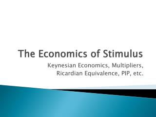
The Economics of Stimulus Keynesian Economics, Multipliers, Ricardian Equivalence, PIP, etc.
Present Value and MEC In the classical model, the business decision maker compared the interest rate to the current marginal productivity of capital: Keynes reminds us of the long life and income stream available from capital, and compares the interest rate to the present value of the future profit stream of the capital. He does this by finding the discount factor d that makes the price of the capital equal to the future stream of income: He then compares d to the interest rate. If d > r, then investment is profitable. The variable d is called the marginal efficiency of capital.
Capital Market Sequence 1.The MEC is contructed. 2.The Money market yields r. 3.The decisionmaker confronts the MEC with r, and makes the investment decision. 4.The resulting investment changes Y and S = S(Y) is determined. Therefore, investment is a function of the supply price of capital, the rate of interest, and long-term expectations. A decline may occur as a result of an increase in PK, an increase in r, or if the MEC collapses as a result of negative expectations about the future. During periods of grossly negative expectations about the future (like the great depression), the investment decision becomes dominated by the expectations term and unresponsive to interest rate changes. The investment schedule becomes quite interest inelastic, so nearly vertical in (I,r)-space.
Investment and the MEC • The MEC is essentially the modern finance concept called the internal rate of return. • The businessperson’s formation of expectations about the future profit stream is pure speculation, and tends to make investment erratic. • Although this is a more sophisticated look at investment than the classicals, still we have that investment depends upon interest rates (and expectations). I = I(r) • Note that I I(Y) and I I(Yd)
45o line Real GDP exceeds planned expenditure 10.0 Total Expenditure C+I+G Aggregate planned expenditure (trillions of 1992 dollars/year) 8.0 f e d 6.0 b c Equilibrium expenditure 4.0 a Planned expenditure exceeds real GDP C0 G I 0 2 4 6 8 10 Real GDP (trillions of 1992 dollars per year)
Stability of the Equilibrium 45o line 10.0 Total Expenditure C+I+G Aggregate planned expenditure (trillions of 1992 dollars/year) 8.0 f Increase Output, increase Employment e d 6.0 Reduce Output, Reduce Employment c b 4.0 a 0 2 4 6 8 10 Real GDP (trillions of 1992 dollars per year)
Algebra of the Model Y = C + I + G but C = C0 + c(Y-T), so Y = C0 + c(Y-T) + I + G Y = C0 + cY – cT + I + G Y – cY = C0 + I + G – cT Y(1-c) = C0 + I + G – cT But this means that but
Multipliers (1) • Thus 1/(1-c) is called the aggregate expenditure multiplier or autonomous expenditure multiplier. • It is positive. • An increase in autonomous spending has a amplified impact on GDP. • But –c/(1-c) is the tax multiplier. • It is negative. • An increase in taxes reduces GDP. • This implies that deficit spending can have a powerful effect for stimulating the economy.
Multipliers (2) • Clearly taxes slow an economy, having a negative effect on GDP and therefore employment. • Note that if G= T, a balanced budget : • Thus the balanced budget multiplier is 1.
Multipliers (3) • As an example, if the mpc = 0.9, then1/(1 – 0.9) = 1/(0.1) = 10 ! • For every $1 increase in government spending, GDP will increase by $10 ! • But also for every $1 that taxes are increased, GDP falls by $9 ! • With a balanced budget (G=T), every $1 increase in G will increase GDP by only $1.
Fiscal Policy Planned Expenditures E1 E0 G Y Y0 Yf
Adding the Foreign Sector • The demand for imports isZ = Z0 + zY, Z0>0, 0<z<1 • Little “z” is the marginal propensity to import. • Exports are thought to be exogenously determined—they don’t depend on conditions in our economy, but rather the conditions in the economy of the buyer nation.
Adapting the Multiplier • Now we have some new components to the multipliers: • Note that we leave out taxes for the moment. • Because the marginal propensity to import is greater than one, the multiplier is now smaller.
Ricardian Equivalence: Assumptions • Agents are rational and farsighted. • Agents either live forever, or care about their progeny as much as they care about themselves. • This implies that agents are linked to the past and the future (by immortality or bequests), and have an infinite time horizon. • The belief that current budget deficits imply future taxes is correct. • Taxes are lump sum. • The availability of the deficit spending does not alter the political process. • No distributional effects. Households are homogeneous, so that a representative agent model can be used. • No liquidity constraints. • Capital markets are perfect.
The Argument (1) • Question: Does it matter whether government finances current spending through taxes or debt? • Assume the gov’t decreases lump-sum taxes in the current period and finances the change with debt:
The Argument (2) • The New Classical Economists argue that agents are not fooled. They recognize that: • In future periods, gov’t will have to pay interest on the additional debt, and • Gov’t will eventually have to repay the debt (assuming it does not have an infinite maturity). • For a given level of gov’t expenditures, the gov’t will have to increase future taxes to pay the debt service and repay the debt.
The Argument (3) • Therefore, households will not view the bonds as an increase in net wealth. • They will subtract the present value of the future taxes from it. • For simplicity, let’s consider a bond of infinite duration:
The Argument (4) • If the bonds and other assets are perfect substitutes, then the subjective discount factor (for time preference in the PV) is equal to the interest rate, and the present value of the tax burden is: • It turns out that the present value of the additional taxes is equal to the debt. • Hence there is no difference between tax and debt finance in terms of the effect on the economy. Gov’t borrowing is not perceived as an increase in private wealth, and consumption demand is not stimulated.
The Argument (5) • Agents increase saving in anticipation of future tax increases. • This causes a reduction in private sector spending that is exactly equal to the increase in government spending. • Deficit spending is not stimulative. It has no effect whatsoever. Thus fiscal policy is useless at best. Activist policy cannot work!
Barro’s Response to Critics • In his later work, Barro makes it clear that he views the “equivalence result” as a benchmark—an extreme case that makes it clear that the effects of deficit spending are not as clear-cut nor as large as Keynesians had suggested.
Policy Ineffectiveness Proposition • How expectations are treated in macro models fundamentally affects the results. • Under rational expectations (endogenous expectations), real output and employment are uneffectedby systematic or predictable changes in aggregate demand policy. • If policy changes are systematic, therefore predictable, then agents will not make systematic mistakes in their forecasts. • Unanticipated policy changes will have a short-run impact.
Phillips Curve under REH inflation LRPC 5 2 4 SRPC(2) 1 3 2 SRPC(1) 1 Unemployment U1 U* SRPC(0)
More on PIP • If a shock to the economy could be anticipated, and if it were to persist, then unanticipated aggregate demand policy could be used to offset its effects. • But if the shock could be anticipated by policymakers, then it could also be anticipated by all agents, and the policy response would also be anticipated and would therefore be ineffective. • Shocks don’t persist (aren’t guaranteed to persist). • Hence there is no role for stabilization policy. • Systematic money supply policy would avoid expectational errors that would likely move the economy temporarily away from full employment. • Therefore, adopt a constant growth rate rule for the money supply.
Time Inconsistency • Kydland and Prescott (1977). “Rules Rather than Discretion: the Inconsistency of Optimal Plans,” JPE. • Because of endogenously formed expectations, optimal policies will not be optimal in practice. • A result of the linear optimal control structure?