Download
1 / 41
410 likes | 512 Vues
This paper explores bridges connecting polygons, including Euclidean and geodesic bridges, recovery schemes for failures, and distributed algorithms. It also discusses optimal bridge solutions for simple polygons and geodesic bridges for point-to-polygon scenarios. The study presents algorithms and results for finding visible bridges and optimal geodesic bridges. Various cases of bridges connecting polygons are analyzed, culminating in the identification of optimal geodesic bridges for simple polygons. The paper concludes by proposing optimal geodesic bridge solutions that can be identified within specific time complexities.

E N D
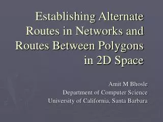
Establishing Alternate Routes in Networks and Routes Between Polygons in 2D Space Amit M Bhosle Department of Computer Science University of California, Santa Barbara
Overview • Bridges connecting polygons • Euclidean bridges: Definition and Results • Geodesic bridges: Definition and Algorithm • Transient failures and proactive recovery schemes • Single link/ node failure recovery (SLFR/SNFR): Problem definitions and our results • Distributed Algorithm: SNFR, SLFR and others • Open Problems
Bridge Connecting Simple Polygons • Two islands, to be connected by a bridge • Flyover-like bridges, and end points need not be visible from each other • Instead of a bridge, we may want to find the route for a ferry that connects the two islands • The (non-amphibian) ferry needs to stay in the water !
Bridge Connecting Simple Polygons • P & Q are two simple, disjoint polygons • Bridge (p, q), with p єρ(P), qєρ(Q) • ρ() defines the region enclosed by the boundary of the polygon • Weight of the bridge (p,q)is: w (p,q) = gd(p, P) + Φ(p,q) + gd(q, Q) • gd(x, X): Geodesic distance between x and its geodesic furthest neighbor in X • Φ(p,q): d(a,b) or gde(p,q), depending on the problem. • Problem asks to find a bridge connecting P and Q which has minimum weight
Simple Polygons: Euclidean Bridges P Q p q gd(p,P) = gd(p,p’) gd(q,Q) = gd(q,q’) p’ q’ w(p,q) = gd(p,P) + d(p,q) +gd(q,Q)
Simple Polygons: Geodesic Bridges P Q p q gd(p,P) = gd(p,p’) gd(q,Q) = gd(q,q’) p’ q’ w(p,q) = gd(p,P) + gde(p,q) + gd(q,Q)
Visible Bridges y y w(opt visible bridge) ~ 2x + 2y w(opt bridge) ~ x + 2y Q x P z An opt bridge’s end points may not be mutually visible: a restriction imposed/assumed in earlier results on the bridge problem Opt visible bridge can be found in O(n log3 n) time. Tan [IJCGA ’02] x >> y >> z
Opt Bridge has End Points on the Polygon Boundaries p q P r Q r’ q’ gd(q,Q) = gd(q,q’) gd(r,Q) = gd(r,r’) • Bridge (p,r)can be shown to be no worse than the bridge (p,q) • gd(r,r’)≤ d(r,q) + gd(q,q’) • Proof holds for geodesic bridges as well
Optimal Bridges: Simple Polygons • We narrow the set of points that can support an optimal bridge to O(n2) anchors on each polygon’s boundary • These O(n2) anchors can be found in O(n2 log n) time • Geodesic furthest point Voronoi Diagram answers the gd(x,X) queries in O(log n) time (can also use Suri’s algorithm [JCCS ’89] to precompute these)
Optimal Euclidean Bridges: Results • An O(n2 log n) time algorithm for the Optimal Euclidean bridge problem • The point to Polygon version of the Euclidean bridge problem can be solved in O(n log n) time • Approximately optimal bridge, within a factor of 1+2/(k+1) of the optimal, in O(kn log n) time • An FPTAS for the Euclidean bridge problem
Geodesic Bridges: Point to Polygon p Q • O(n2) candidate bridge end points on Q • Build the SP tree of p to all the O(n2) points in O(n2 log n)time using Hershberger and Suri’s algorithm [SIAM J. ’99] • Precompute geodesic furthest neighbors of each of the O(n2) points in O(n2 log n) time q’ q Works. But for the 2 polygon case, will need ~ O(n4)time (since we have O(n2) anchors on each polygon)
Geodesic Bridges: Point to Polygon p q Q • Either (p,q) is a visible bridge • Can be found in O(n logn) time q0 q • OR • The 2nd last vertex of gd(p,q) (q0in fig) is a • vertex of Q. • And, (q0 ,q) is optimal visible bridge from q0to Q (sub-path optimality)
Optimal Geodesic Bridge: Point to Polygon • From p and each vertex of Q, precompute the optimal visible bridge to Q in O(n2 log n) total time • From p, find the shortest paths to all vertices of Q: O(n log n) time • Select best among vis(p,Q) and MIN q єV(Q){gd(p,q) + vis(q,Q)} • Total of O(n2 log n) time
Geodesic Bridges: Simple Polygons P Q p q Case I: (p,q) is a one-link bridge => (p,q) is a visible bridge. An optimal visible bridge between P and Q can be found in O(n log3 n) time using Tan’s algorithm.
Geodesic Bridges: Simple Polygons P Q q p x • Case II: (p,q) is a two-link bridge, pivoted at a vertex, say x • (x, p) is an optimal visible bridge from x to P • (x, q) is an optimal visible bridge from x to Q • There are a total of 2n such bridges, that can be found in O(n2 log n) total time
Geodesic Bridges: Simple Polygons q0 P Q q p p0 • Case III: (p,q) is a multi-link bridge • the second and second-last vertices of gde(p,q), p0and q0, are vertices of P and/or Q • (p0 , p) is an optimal visible bridge from p0to P • (q0 , q) is an optimal visible bridge from q0to Q • There are a total of O(n2)such bridges, that can be found in O(n2 log n) total time
Optimal Geodesic Bridges: Simple Polygons • Each of the three types of bridges, one-link, two-link and multi-link, can be found in O(n2 log n) time or less. The best among them is an optimal geodesic bridge between the two polygons. • Therefore, we can find an optimal geodesic bridge in O(n2 log n) time • The time bound matches our bound for finding an optimal Euclidean bridge between two simple polygons • The point to Polygon version of the geodesic bridge problem can be approximated to a factor of 1+2/(k+1) in O(kn log n) time
Some Open Problems Related to Bridges • Faster exact algorithms for the optimal Euclidean bridge and optimal geodesic bridge problems? • o(n2)-time approximation algorithms for the geodesic bridge problem?
Failures in IP Backbones • Five 9s availability (99.999% uptime) is highly desirable • VOIP, VPN, Banking, Multimedia Conferencing, Shopping, … • Failures occur quite frequently • Faulty interfaces, router/link failures, maintenance activity • Markopolu, et al. (INFOCOM 2004) characterized the failures in IP backbones • About 20% failures due to planned activity (e.g. maintenance) • Most unplanned failures in communication networks are transient and affect a single element • 46% last less than 1 minute • 86% last less than 10 minutes • 85% of all failures affect a single link or node • Handling transient single node or link failures is key to ensuring high availability
Proactive Recovery Schemes • Popular technique of handling transient failures • Precompute alternate paths that avoid the failed element • When a failure actually occurs • Suppress the failure, instead of the traditional approach of advertising it across the network (and hope that it is a transient issue) • Use the precomputed alternate paths to reroute traffic (and survive the failure)
Single Link Failure Recovery (SLFR) • Given an edge weighted graph G (V,E), and the shortest paths tree Ts = {e1 , e2 ,…, en-1}of a node s, where ei= {xi , yi} and xi is the parent of yiin Ts • For 1 ≤ i ≤ n-1, find the shortest path from yi to s in the graph G-i = G \ ei • G-i is obtained from G by deleting the edge ei • G assumed to be 2-edge-connected, and undirected
Single Node Failure Recovery (SNFR) • Given an edge weighted graph G(V,E), and the shortest paths tree Tsof a node s, where Cx= {x1 , x2 , x3 ,…, xk}denote the children of x in Ts • For each node x є G, and x ≠ s, find a path from each xiєCxto s in the graph G-x = (V \ x, E \ Ex) • G-x is obtained from G by deleting the node x and all its edges • G assumed to be 2-node-connected, and undirected
SLFR SNFR s s x x y xi xj xk
SLFR, SNFR: Naïve Algorithm • Recompute the shortest paths tree of s separately in each of the n-1 failure graphs (G-igraphs for SLFR problem, and G-xgraphs for SNFR problem) • Time Complexity: Since we have O(n)failure graphs, the naïve algorithm requires O(n(m+nlog n))time • Simple, but inefficient (at least for undirected graphs)
SLFR, SNFR: Our Results (Centralized Algorithms) • SLFR: O(m + nlog n)time for computing optimal alternate paths • Undirected, planar graphs: linear time • Undirected, integer edge weights: O(m + Tsort(n)) • Some improvements for replacement-paths problem • Given an s-t shortest path, find alternate s-t paths if each edge of the original s-t shortest path fails, one at a time • SNFR: O(m log n)time algorithm • Computes good alternate paths – within 15% of optimal for randomly generated graph with 100 – 1000 nodes, and an average degree of 10 – 30 • Protocols: A new proactive recovery scheme that uses the paths computed by these algorithms to recover from transient single element failures
Single Node Failure Recovery:A Distributed Algorithm? • All previous algorithms, including our earlier algorithms, are centralized algorithm that need complete information of the Network graph as input to the algorithms • Resource intensive – need a single computer with enough processing power, and memory to deal with potentially huge network graphs • Manually intensive • Need a consistent snapshot of the network • Results of the computation need to be deployed to the corresponding hosts • Especially desirable if the other steps performed at the Network setup are distributed algorithms • Thesis proposal question – can our ideas from the centralized algorithms be used for designing a distributed algorithm for computing alternate paths?
SNFR: Key Properties s G x xj xi x1 gj bq bp gi • Green edges (e.g. gi, gj) have one end point outside the subtree of x. • giand gjcan be used by xiand xj respectively to reach s. • Blue edges (e.g. bp, bq) run between subtrees of siblings. • Together with green edges, they can offer a valid alternate paths. • E.g. bpoffers an alternate path to x1(either bq gj, or directly using gi).
SNFR: Constructing Rx s G x xj x1 xi gj bq bp gi sx sx yi yj y1 yi yj y1 Rx Tsx
SNFR • Each node needs the following information • Cheapest green edge for each child node • Blue edges among the subtrees of the child nodes • An edge is green for a node if it has one end point in the node’s subtree, and the other outside the node’s parent’s subtree • An edge is blue in Rx if x is the nearest-common-ancestor of the two end points of the edge
DFS Start / End Labels (1,14) (12,13) (2,11) u w (5,10) (3,4) (8,9) (6,7) v • Assign start and end labels to nodes as a depth-first-search traversal of the tree starts or ends at the node • A node v belongs to the subtree of u iff dfsStart(u) < dfsStart(v) < dfsEnd(v) < dfsEnd(u) • Green edges have exactly one end point in the node’s subtree
Distributed SNFR: Gathering Information to Construct Rx (1,200) s (2,101) x (102, 199) xi (3,50) xj (51,100) b v u (80,91) (10,21) • M(u,v): • (10,21) – (80,91) • loop weight: d(s,u) + cost(u,v) + d(v, s)
Distributed SNFR: Gathering Information to Construct Rx (1,200) s (2,101) x (102, 199) xi (3,50) xj (51,100) z b v g (110,151) u y (60,71) • M(y,z): • (60,71) – (110,151) • loop weight: d(s,y) + cost(y,z) + d(z, s) Forward a child node’s edge to your parent if and only if it is a green edge
Distributed SNFR Algorithm • DFS labels computed using the algorithm by Fraigniaud, et. al. [PODC ’00] • The root node, s, initiates the SNFR algorithm by sending a control message to all nodes – asking them to start forwarding their non-tree edges • After a leaf node has forwarded all its non-tree edges, it sends a special DONE message to its parent to indicate that it has finished fwd’ing all non-tree edges • An intermediate node sends a DONE message to its parent after it is done, and it has received DONE from all its children • Once a node x has received DONE from all its children, it has enough information to construct Rxlocally, and finish the remaining steps of the alternate path computation algorithm
Distributed SNFR Algorithm: Summary • First distributed algorithm for computing alternate paths • Based on request-response model – does not need any global coordination among the nodes • Requires O(m+n)messages to be transmitted among the nodes, and has a space complexity of O(m+n)across all nodes (asymptotically optimal) • Can be generalized to the Single Link Failure Recovery and a few other related problems.
Some Open Problems Related to SLFR/SNFR • Faster algorithm and/or better alternate paths for SNFR problem • Our solution runs in O(m log n) time, and does not compute optimal alternate paths • Naïve upper bound for computing optimal alt paths: O(n(m + n log n)) • Directed graphs • Our upper bounds are strictly for undirected graphs • (m n) lower bound holds for directed graphs in path comparison model (as long as m = O(n n) ) • Recently, replacement paths problem solved in O(n log3n) time for directed planar graphs [EPR ’08] • Multiple failures • Failure of any two links or nodes in the network? We presented an O(n3) algorithm for computing alternate s-t paths when the 2 failed links or nodes are on the original s-t path • Trivial lower bound of (n2)
O(n log n)Algorithm for Optimal Vertex Bridge • Vertex bridge is between the vertices of the 2 polygons • Additively weighted nearest-point Voronoi diagram • Each Voronoi point u has an associated weight wv • Query for point p returns a point v such that d(p, v) + wv = MIN u є V{d(p,u) + wu} • Can be built in O(n log n) time [Aurenhammer-Imai ’88] • Query can be answered in O(log n) time • Geodesic furthest neighbors of all vertices of a simple polygon can be found in O(n log n) time [Suri ’89]
Optimal Vertex Bridge (Contd.) • For each vertex q є Q, assign weight wq = gd(q, Q) • O(n log n) total time • For each vertex p є P, find the vertex q є Q with minimum d(p, q) + wq • This would be the best vertex bridge with p as one end point • Each query in O(log n) time • Check all vertices of P for the optimal vertex bridge • Total time O(n log n)