### Effective Decision Making Through Simulation in Economics ###
Welcome to AGEC 622! I am James Richardson, your instructor for the semester. Jing Yi will be your grader and Brian Herbst will assist in the labs. This course focuses on Decision Making under Risk, exploring systematic methods for evaluating potential outcomes and their probabilities. We will discuss forecasting, risk management, and simulations, which are vital tools for analyzing risky decisions. Understand how to apply econometric models to real-world scenarios, considering risk in economic analysis to improve your decision-making skills. ###

### Effective Decision Making Through Simulation in Economics ###
E N D
Presentation Transcript
AGEC 622 • I am James Richardson • I get to be your teacher for the rest of the semester • Jing Yi will be the grader for this section. • Brian Herbst will assist in the Labs • If you have problems with homeworks see Jing, Brian, or me • Are you attending the labs? • Lab is not required, but highly recommended
Courseis about Decision Making • How do you make decisions? • Do you list all of the possible outcomes and their consequences? • Do you think about the probabilities for each possible outcome? P(win) = 25% • Do you fixate on the outcome you want? P(win) = 100% • Do you just go through life without planning? • Systematic consideration of options • Consider probabilities of choices • What ever …..
Topics I cover & their application to life • Topics: forecasting, risk management, and decision making under risk • If you live you are faced with decisions • Decisions you make affect how, and how well you live; and will have consequences forever • Every decision you make has risk • In business, simulation is the tool we use to analyze risky decisions • It is used in business, government, and academia • You already use it, ifyou think through possible outcomes for a decision
Simulation for Ag Economists • Apply econometric equations for forecasting under risk • Valuing new technology under risk • Test alternative business management plans with risk • Assess the potential for profits with a new business with risk • Common theme here is – RISK and MONEY • Everything we do has risk
20% Return Y 30% Return X Application of Risk in a Decision • Given two investments, X and Y • Both have the same cash outlay • Return for X averages 30% • Return for Y averages 20% • If no risk then invest in alternative X
X -20 -10 0 10 20 30 40 50 Y Application of Risk in a Decision • Given two investments, X and Y • Cash outlay same for both X and Y • Return for X averages 30% • Return for Y averages 20% • What if the distributions of returns are known as: • Simulation estimates the shape of the distribution for returns on risky alternatives 0 10 20 30 40 50 60 70 80 90
Simulation Models and Decision Making • Start with a problem that includes risk • Identify risky variables and control variables you can change (scenarios) • Gather data, estimate regressions, and develop equations for model • Generally these are accounting equations, e.g. Profit = Revenue – Variable and Fixed Costs • Simulate model under risk • Analyze results and make decisions for best scenario
Purpose of Simulation • … to estimate distributions that we can not observe and apply them to economic analysis of risky alternatives (strategies) so the decision maker can make better decisions • Profit = (P * Ỹ) – FC – (VC * Ỹ) ~ ~ ~
Two Quotes to Start this Section 622 • “My job is not to be easy on people. My job is to make people better.” Steve Jobs 2008 • “Let’s go do something today rather than dwell on yesterdays mistakes.” JWR 2012 • In computer modeling and simulation you learn by making mistakes, expect to make mistakes • To learn from your mistakes, you have to figure out how to correct them • After learning how to fix a mistake move on and prosper
Materials for This Lecture • Read Chapter 16 of Simulation book • Read Chapters 1 and 2 • Read first half of Chapter 15 on trend forecasting • Read journal article “Including Risk in Economic .. • Readings on the website • Richardson and Mapp • Including Risk in Economic Feasibility Analyses … • Before each class review materials on website • Demo for the days lecture • Overheads for the lecture • Simulation Book is on the website
Forecasting and Simulation • Forecasters give a point estimate of a variable • Because we use simulation, we will use probabilistic forecasting • This means we will include risk in our forecasts for business decision analysis
Simulate a Forecast • Two components to a probabilistic forecast • AGEC 621 taught you how to develop a deterministic component forecast. It gives a point forecast: Ŷ = a + b1 X + b2 Z • Stochastic componentẽ was ignored it is used as: Ỹ = Ŷ + ẽ Which leads to the complete probabilistic forecast model Ỹ = a + b1 X + b2 Z + ẽ • ẽ makes the deterministic forecast a probabilistic forecast
Steps for Probabilistic Forecasting • Simulation provides an easy method for incorporating probabilities and confidence intervals into forecasts • Steps for probabilistic forecasting • Estimate best econometric model to explain trend, seasonal, cyclical, structural variability to get ŶT+i • Residuals (ê) are unexplained variability or risk; an easy way is to assume ê is distributed normal • Simulate risk as ẽ = NORM(0,σe) • Probabilistic forecast is ỸT = ŶT+i + ẽ or ỸT = ŶT+i + NORM(0,σe)
Major Activities in Simulation Modeling • Estimating parameters for probabilistic forecasts • Ỹt = a + b1Xt + b2Zt + b3 Ỹt-1 + ẽ • The risk can be simulated with different distributions, e.g. • ẽ = NORMAL (Mean, Std Dev) or • ẽ = BETA (Alpha, Beta, Min, Max) or • ẽ = Empirical (Sorted Values) or others • Estimate parameters (a b1 b2 b3), calculatethe residuals (ê) and specify the distribution for ê • Simulate random values from the distribution (Ỹt) • Validate that simulated values come from their parent distribution • Model development, verification, and validation • Apply the model to analyze risky alternatives and decisions • Statistics and probabilities • Charts and graphs (PDFs, CDFs, StopLight) • Rank risky alternatives
Role of a Forecaster • Analyze historical data series to quantify patterns that describe the data • Extrapolate the pattern into the future for a forecast using quantitative models • In the process, become an expert in the industry so you can identify structural changes before they are observed in the data – incorporate new information into forecasts • In other words, THINK • Look for the unexpected
Types of Forecasts • There are several types of forecast methods, use best method for problem at hand • Three types of forecasts • Point or deterministic Ŷ = 10.0000 • Range forecast Ŷ = 8.0 to 12.0 • Probabilistic forecast • Forecasts are never perfect so simulation is a way to protect your job
Forecasting Tools in AGEC 622 • Trend • Linear and non-linear • Multiple Regression • Seasonal Analysis • Moving Average • Cyclical Analysis • Exponential Smoothing • Time Series Analysis
Define Data Patterns • A time series is a chronological sequence of observations for a particular variable over fixed intervals of time • Daily • Weekly • Monthly • Quarterly • Annual • Six patterns for time series data (data we work with is time series data because use data generated over time). • Trend • Cycle • Seasonal variability • Structural variability • Irregular variability • Black Swans
Trend • Trend a general up or down movement in the values of a variable over a historical period • Most economic data contains at least one trend • Increasing, decreasing or flat • Trend represents long-term growth or decay • Trends caused by strong underlying forces, as: • Technological changes, eg., crop yields • Change in tastes and preferences • Change in income and population • Market competition • Inflation and deflation • Policy changes
Simplest Forecast Method • Mean is the simplest forecast method • Deterministic forecast of Mean Ŷ = Ῡ = ∑ (Yi ) / N • Forecast error (or residual) êi = Yi – Ŷ • Standard deviation of the residuals is the measure of the error (or risk) for this forecast σe = [(∑(Yi – Ŷ)2/ (N-1)]1/2 • Probabilistic forecast Ỹ = Ŷ + ẽ where ẽ represents the stochastic (risky) residual and is simulated from the êiresiduals
Linear Trend Forecast Models ^ ^ • Deterministic trend model ŶT= a + b TT where Tt is time; it is a variable expressed as: T = 1, 2, 3, … or T = 1980, 1981, 1982, … • Estimate parameters for model using OLS • Multiple Regression in Simetar is easy, it does more than estimate a and b • Std Dev residuals & Std Error Prediction (SEP) • When available use SEP as the measure of the error (stochastic component) for the probabilistic forecast • Probabilistic forecast of a trend line becomes Ỹt = Ŷt + ẽ Which is rewritten using the Normal Distribution for ẽ Ỹt = Ŷt+ NORM(0, SEPT) where T is the last actual data ^ ^
Non-Linear Trend Forecast Models ^ ^ ^ ^ • Deterministic trend model Ŷt = a + b1Tt+ b2 Tt2+ b3 Tt3 where Tt is time variable is T = 1, 2, 3, … T2 = 1, 4, 9, … T3 = 1, 8, 27, … Estimate parameters for model using OLS • Probabilistic forecast from trend becomes Ỹt = Ŷt+ NORM(0, SEPT)
Steps to Develop a Trend Forecast • Plot the data • Identify linear or non-linear trend • Develop T, T2, T3 if necessary • Estimate trend model using OLS • Observing a low R2 is a usual result • F ratio and t-test will be significant if trend is statistically present • Simulate model using Ỹt= Ŷt+ NORM(0, SEPT) • Report probabilistic forecast
Linear Trend Model • F-test, R2, t-test and Prob(t) values • Prediction and Confidence Intervals
Non-Linear Trend Regression • Add square and cubic terms to capture the trend up and then the trend down
Is a Trend Forecast Enough? • If we have monthly data, the seasonal pattern may overwhelm the trend, so final model will need both trend and seasonal terms (See the Demo for Lecture 1 ‘MSales’ worksheet) • If we have annual data, cyclical or structural variability may overwhelm trend so need a more complex model • Bottom line • Trend is where we start, but we generally need a more complex model
Types of Forecast Models • Two types of models • Causal or structural models • Univariate (time series) models • Causal (structural) modelsidentify the variables (Xs) that explain the variable (Y) we want to forecast, the residuals are the irregular fluctuations to simulate Ŷ = a + b1 X + b2 Z + ẽ Note: we will be including ẽ in our forecast models • Univariate models forecast using past observations of the same variable • Advantage is you do not have to forecast the structural variables • Disadvantage is no structural equation to test alternative assumptions about policy, management, and structural changes Ŷt = a + b1Yt-1 + b2 Yt-2 + ẽ ^ ^ ^ ^ ^ ^
Meaning of the CI and PI • CI is the confidence for the forecast of Ŷ • When we compute the 95% CI for Y by using the sample and calculate an interval of YL to YU we can be 95% confident that the interval contains the true Y0. Because 95% of all CI’s for Y contain Y0 and because we have used one of the CI from this population. • PI is the confidence for the prediction of Ŷ • When we compute the 95% PI we call a prediction interval successful if the observed values (samples from the past) fall in the PI we calculated using the sample. We can be 95% confident that we will be successful.
Confidence Intervals in Simetar Beyond the historical data you will find: SEP values in column 4 Ŷ values in column 2 Ỹ values in column 1