Particle Size Analysis
Particle Size Analysis. How do we define particle size? In class exercise Some of the many different ways Use of fractal dimension to describe irregular shapes. Particle size . Simplest case: a spherical, solid, single component particle Critical dimension: radius or diameter

Particle Size Analysis
E N D
Presentation Transcript
Particle Size Analysis • How do we define particle size? • In class exercise • Some of the many different ways • Use of fractal dimension to describe irregular shapes
Particle size Simplest case: a spherical, solid, single component particle Critical dimension: radius or diameter Next case: regular shaped particles Examples Shape Dimensions NaCl crystals cubes side length More complicated: irregular particles Appropriate particle size characteristic may depend on measurement technique (2-D images, measuring sedimentation velocity, light scattering, sieving, electrical mobility, surface area measurements etc..)
Particle size from image analysis Optical and electron microscopes give 2-D projected images of particles (3-D objects) The irregular particle Equivalent circle diameter Diameter of circle with equivalent projected area as particle Enclosing circle diameter Diameter of circle containing projected area Martin’s diameter Length of line bisecting projected area (a given particle could have a range) Shear diameter How far you must move the particle so that it is not overlapping its former position (could this also have range?)
Radius of Gyration “The Radius of Gyration of an Area about a given axis is a distance k from the axis. At this distance k an equivalent area is thought of as a Line Area parallel to the original axis. The moment of inertia of this Line Area about the original axis is unchanged.” http://www.efunda.com/math/areas/RadiusOfGyrationDef.cfm
Particle size- equivalent diameters • Other equivalent diameters can be defined: • Sieve equivalent diameter – diameter equal to the diameter of a sphere passing through the same sieve aperture as particle • Surface area equivalent diameter – diameter equal to diameter of a sphere with same surface area as particle • Aerodynamic diameter – diameter of a unitdensity sphere having the same terminal settling velocity as the particle being measured • This diameter is very important for describing particle motion in impactors, and cyclone separators. In shear flows though, describing the motion of irregular particles is a complex problem and it may not be possible to describe their motion by modeling their aerodynamic spherical equivalents.
More diameters • Volume diameter – diameter of sphere having same volume • Obtained from Coulter counter techniques • Surface volume diameter – diameter of sphere having same surface to volume ratio • Obtained from permeametry (measuring pressure drop with flow through a packed bed) • Mobility diameter – diameter equal to the diameter of a sphere having the same mobility in an electric field as particle
Concept of fractal dimension • Aerosol particles which consist of agglomerates of ‘primary particles’, (often, combustion generated) may be described using the concept of fractals. • Fractals - The relationship between radius r (rgyration usually) of aerosol agglomerates, and the volume of primary particles in the agglomerate can be written:
Fractal dimension • Fractals - Df = 2 = uniform density in a plane, Df of 3 = uniform density in three dimensions. • Typical values for agglomerates ranges from 1.8 to near 3 depending on mechanism of agglomeration and possible rearrangement.
Particle Size Con’t • Particle concentration – suspensions in air • Particle density – powders • What if particles are not all the same size? • Size distribution – discrete and continuous • Number, volume and mass based distributions • Frequency distributions • Histogram tricks • Single modes – different types of averaging • Moments
Particle concentration Again, many different ways to describe concentration Low concentrations of suspended particles: usually number, mass or volume concentrations are used Number concentration = number of particles/ unit volume of gas V = volume of particles containing N particles Deviation due to small particle number Deviation due to spatial variation of concentration P Particle concentration Region in which particle concentration is defined Size of region V
Mass and Volume Concentrations Mass concentration: particle mass per unit volume of gas Volume concentration: particle volume per unit volume of gas If all particles are the same size, simple relationships connect number, mass and volume concentrations (exercise): Number concentrations important for clean rooms. Class 1 = less than 1000 0.1 micron diameter particles per m3, ambient ranges from 10^3 to 10^5 per cm3. Mass concentrations usually reported as g/m3 of gas. Typical ambient concentrations: 20 g/m3 for relatively clean air, 200 g/m3 for polluted air. Volume concentration can be related to ppm by volume, dimensionless. Used mainly only for modeling.
Particle concentrations - powders Additional definitions necessary: Bed or bulk density = mass of particles in a bed or other sample volume occupied by particles and voids between them Tap density = density after being “packed”, mass/volume, very arbitrary!!! (think about cereal) Void fraction = volume of voids between particles volume occupied by particles and voids between them
What if we have a mixture of particles of different sizes? In the real world, this is most often the case. Monodisperse – all particles are the same size Polydisperse – the particles are of many different sizes How do we describe this? Using a size distribution. Distributions can be discrete or described by a continuous function. Discrete distributions can be represented well using histograms. Discrete example: you are given a picture of 1000 spherical particles, of size ranging from 1 to 100 microns. You measure each particle diameter, and count the number of particles in each size range from 0 to 10 microns, 10 to 20 microns etc.. Size ranges are often called ‘bins’.
Example histogram: Can also create histogram from raw particle size data using Analysis tool pack add-in, with Excel.. After add-in, go to ‘tools’, then ‘data analysis’, then ‘histogram’.
Continuous particle size distributions More useful: continuous distributions, where some function, nd, describes the number of particles of some size (dp, or x in Rhodes), at a given point, at a given time. In terms of number concentration: Let dN = number of particles per unit volume of gas at a given position in space (represented by position vector r), at a given time (t), in the particle range d to dp + d (dp). N= total number of particles per unit volume of gas at a given position in space at a given time. Size distribution function is defined as: nd(dp, r, t) = dN d(dp) Can also have size distribution function, n, with particle volume v as size parameter: n(v, r, t) = dN (not as common) dv In this case, what does dN represent?
More continuous size distributions M is total mass of particles per unit volume at a given location, r, at a given time, t. The mass of particles in size range dp to dp+d(dp) is dM. Mass distribution function m is: V is total volume of particles per unit volume at a given location, r, at a given time, t. The volume of particles in size range dp to dp+d(dp) is dV. Volume distribution function is: nd(dp) and n(v) can be related: Where does this come from? How can m (dp,r,t) and v (dp,r,t) be related?
Frequency distributions Cumulative frequency distribution: FN = fraction of number of particles with diameter (Fv for volume, Fm for mass, Fs for surface area) less than or equal to a given diameter. In Rhodes, F is by default FN. Can obtain cumulative frequency distribution from discrete data Derivative of cumulative frequency distribution with respect to particle diameter is equal to the differential frequency distribution. Differential frequency distribution is a normalized particle size distribution function. d FN /d(dp) = fN(dp) = 1dN Nd(dp) d FN /d(dp) = fN(dp) = 1dV = 1 dM V d(dp) M d(dp)
Example of cumulative frequency distribution from discrete data Example of differential frequency distribution in Fig. 3.3 Rhodes
More on size distributions In measuring size distributions, instruments such as impactors give mass of particles for a particular size bin (more on exactly how impactors work later). Because of spread in size over many orders of magnitude, log scale often used for x axis (diameter). Often data are presented as dM/ d(log dp) versus log dp. This way, area for each bar in special histogram is proportional to mass of particles in that size class.
Number, mass, surface area distributions not the same! • Mass distribution from before Using arithmetic average of min and max bin diameter, I created a number distribution Where did the second peak go?
Describing distributions using a single number, a.k.a. what is average? General formula for the mean, x, of a size distribution: g is the weighting function. F is the cumulative frequency distribution. F g(x) g(x) Definitions of other means Mean, notation weighting function g(x) Quadratic mean, xq x2 Geometric mean, xg log x Harmonic mean xh 1/x
Standard shapes of distributions Normal Log normal Bimodal
Similarity transformation The similarity transformation for the particle size distribution is based on the assumption that the fraction of particles in a given size range (ndv) is a function only of particle volume normalized by average particle volume: defining a new variable, and rearranging,
Self-preserving size distribution For simplest case: no material added or lost from the system, V is constant, but is decreasing as coagulation takes place. If the form of is known, and if the size distribution corresponding to any value of V and is known for any one time, t, then the size distribution at any other time can be determined. In other words, the shapes of the distributions at different times are similar, and can be related using a scaling factor. These distributions are said to be ‘self-preserving’. t1 t2 t3