Consumption Function – I
Consumption Function – I. ECN Data Analysis Lawlor. Macroeconomic Time Series. Data issue is to consider the nature of economic series that move through time These are typically “dated” Annually, quarterly, monthly In economics these are often Macroeconomic data History only happened once.

Consumption Function – I
E N D
Presentation Transcript
Consumption Function – I ECN Data Analysis Lawlor
Macroeconomic Time Series • Data issue is to consider the nature of economic series that move through time • These are typically “dated” • Annually, quarterly, monthly • In economics these are often Macroeconomic data • History only happened once
Consumption Function • Our example of this will be the estimation of a “Consumption Function” • For the United States in the post-war period • Only years for which we have data • Requires a very little bit of background in Macroeconomic theory
Formal Theory of the Cons. Fn. • Specifies the nature of the determinants of real aggregate household consumption (C). • Asserts the major determinant of this in short-run data (say quarterly or monthly) is contemporaneous real income (Y) • Describes this in the form of a general function: • C = f(Y,…)
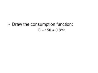
Many attempts to estimate in many data contexts • 1st. step is to linearize the relation • So we can use simple regression • C = a + b*Y • Where, • a = intercept of cons function, sometimes interpreted as “autonomous consumption” • that part of C not caused by changes in Y • “b” = the slope of the consumption function • sometimes interpreted as “induced consumption” • that part caused by changes in Y
Data derived Cons. Fn. • If you were to display the contemporaneous data on C and Y on a scatterplot… • Do so on Gretl • Show on board • Derive: MPC, MPS, a • One of the most stable relationships in economics
Show how data implies “the fundamental psychological law: • This form of the “fundamental psychological law” • 0 < a • 0 < b, or MPC < 1 • Says that, in the short-run, “when household income increases, so does household consumption, but not by as much” • Again, 0 < MPC < 1
Now look at origin of Cons. Fn. • JMK, writing in the Great Depression • Reading Keynes: • Choice of units • Discussion of the precision with which macroeconomic time series data are measured • Can we really rely on aggregate P and Y the over long-period? Think how we define real C and real Y. • JMK says no, reason we should confine macroeconomics, an macroeconomics to the short-run- say a decade, or the time span between usual business cycles
JMK on the “Propensity to Consume” • pp. 12-14 in text selection • States a verbal form of “fundamental psychological law” • namely that people are disposed to “increase their consumption as their income increases, but not by as much as the increase in their income.” • Says the MPC is “positive and less than unity” • Note, for us, this importantly corresponds to the data of repeated attempts to estimate the cons. fn.
Two additional hints from JMK, worth storing away for later study • 1. He suggests that many other factors may co-determine the consumption levels of different countries • Seen today in wildly different MPC’s across the globe • His choice for the most important measurable variable is “windfall changes in capital values” • 2. He suggest MPC may fall at as Y drifts higher
Keynes and the Data • Use Gretl – “Browse Databases” • Explore and install various series from the St. Louis Federal Reserve • Want to find and open variables that measure C and Y • In series “find” window search for “consumption” and “income” • Looking for “real” personal consumption and disposable income of households
Plot and explore the Data • Note first the nature of the data: monthly, real, seasonally adjusted, from 1959:01 to 2007:06 • Highlight both and display as “time series plot” • Note how good it fits our conception of “fund. psych. law” • Note we can use the mouse to figure out what year we are looking at • Note it is over “long-run” data from 1959 to present – should this be a problem?
Explore, contd. • Note you can “zoom” in on a particular time period in the “edit” menu • Show it in a “scatterplot” • Comment on the “line of best fit” • Note the value of the intercept, pos., neg, O • Select “Model” and estimate an “OLS” regression • Interpret the coefficients and output
The Cons. Fn. And the U.S. “Great Depression” • Think of the historical context • Great uncertainty about employment, extreme frugality • Why? As seen in figs. on 4, a collapse of Y and C and I • Fig. 11 on p. 5, shows the stability of spending on consumption versus the excessive volatility of investment
Estimate a Cons. Fn. For these years • Last page shows this • First figure is the material out of which a consumption function is made • notice C > Y in 1932-1934 • Think about that and annual data (all available) • Now run the regression: results graphically displayed in second figure • Note the very high MPS, = .76