Presentation Transcript

1. Lecture 2: linear algebra, animation basics

   Computer Animation

2. Vector Arithmetic
3. Vector Magnitude The magnitude (length) of a vector is: Unit vector (magnitude=1.0)
4. Dot Product
5. Example: Angle Between Vectors How do you find the angle θ between vectors a and b? b θ a
6. Example: Angle Between Vectors b θ a
7. Dot Products with Unit Vectors 0 <a·b < 1 a·b = 0 a·b = 1 b θ a -1 < a·b < 0 a·b a·b = -1
8. Dot Products with Non-Unit Vectors If a and b are arbitrary (non-unit) vectors, then the following are still true: If θ < 90º then a·b > 0 If θ = 90º then a·b = 0 If θ > 90º then a·b < 0
9. Dot Products with One Unit Vector If |u|=1.0 then a·u is the length of the projection of a onto u a u a·u
10. Cross Product
11. Properties of the Cross Product area of parallelogram ab if a and b are parallel is perpendicular to both a and b, in the direction defined by the right hand rule
12. Example: Area of a Triangle Find the area of the triangle defined by 3D points a, b, and c c b a
13. Example: Area of a Triangle c c-a b a b-a
14. Example: Alignment to Target An object is at position p with a unit length heading of h. We want to rotate it so that the heading is facing some target t. Find a unit axis a and an angle θ to rotate around. t • • p h
15. Example: Alignment to Target a t t-p • θ • p h
16. Trigonometry cos2θ+ sin2θ= 1 1.0 sin θ θ cos θ
17. Laws of Sines and Cosines Law of Sines: Law of Cosines: b α γ c a β
18. Matrices Computer graphics apps commonly use 4x4 homogeneous matrices A rigid 4x4 matrix transformation looks like this: Where a, b, & c are orthogonal unit length vectors representing orientation, and d is a vector representing position
19. Matrices The right hand column can cause a projection, which we won’t use in character animation, so we leave it as 0,0,0,1 Some books store their matrices in a transposed form. This is fine as long as you remember that: (A·B)T = BT·AT
20. Orthonormality If all row vectors and all column vectors of a matrix are unit length, that matrix is said to be orthonormal This also implies that all vectors are perpendicular to each other Orthonormal matrices have some useful mathematical properties, such as: M-1 = MT
21. Orthonormality If a 4x4 matrix represents a rigid transformation, then the upper 3x3 portion will be orthonormal
22. Determinants The determinant of a 4x4 matrix with no projection is equal to the determinant of the upper 3x3 portion
23. Determinants The determinant is a scalar value that represents the volume change that the transformation will cause An orthonormal matrix will have a determinant of 1, but non-orthonormal volume preserving matrices will have a determinant of 1 also A flattened or degenerate matrix has a determinant of 0 A matrix that has been mirrored will have a negative determinant
24. Transformations To transform a vector v by matrix M: v’=v·M If we want to apply several transformations, we can just multiply by several matrices: v’=(((v·M1)·M2)·M3)·M4… Or we can concatenate the transformations into a single matrix: Mtotal=M1·M2·M3·M4… v’=v·Mtotal
25. Matrix Transformations We usually transform vertices from some local space where they are defined into a world space v’ = v·W Once in world space, we can perform operations that require everything to be in the same space (collision detection, high quality lighting…) Then, they are transformed into a camera’s space, and then projected into 2D v’’ = v’·C-1·P In simple situations, we can do this all in one step: v’’ = v·W·C-1·P
26. Inversion If M transforms v into world space, then M-1 transforms v’ back into local space
27. Vector Dot Vector
28. Vector Dot Matrix
29. Matrix Dot Matrix
30. Homogeneous Vectors Technically, homogeneous vectors are 4D vectors that get projected into the 3D w=1 space
31. Homogeneous Vectors Vectors representing a position in 3D space can just be written as: Vectors representing direction are written: The only time the w coordinate will be something other than 0 or 1 is in the projection phase of rendering, which is not our problem
32. Position Vector Dot Matrix
33. Position Vector Dot Matrix y v=(.5,.5,0,1) x (0,0,0) Local Space
34. Position Vector Dot Matrix b Matrix M y y d a v=(.5,.5,0,1) x x (0,0,0) (0,0,0) Local Space World Space
35. Position Vector Dot Matrix b v’ y y d a v=(.5,.5,0,1) x x (0,0,0) (0,0,0) Local Space World Space
36. Direction Vector Dot Matrix
37. Matrix Dot Matrix (4x4) The row vectors of M’ are the row vectors of M transformed by matrix N Notice that a, b, and c transform as direction vectors and d transforms as a position
38. Identity Take one more look at the identity matrix It’s a axis lines up with x, b lines up with y, and c lines up with z Position d is at the origin Therefore, it represents a transformation with no rotation or translation

39. Animation basics

40. Animation Process while(!finished) { UpdateEverything(); DrawEverything(); } Interactive vs. Non-Interactive Real Time vs. Non-Real Time
41. Frame Rates Film 24 fps Imax 48 fps NTSC TV 30 fps (interlaced) PAL TV 25 fps (interlaced) HDTV 50-60 fps Computer >60 fps
42. Animation Tools Animation tools: Maya 3D Studio Max MotionBuilder Blender Game/graphics engines: OGRE3D Unity Unreal
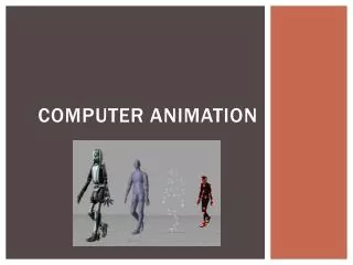
43. Virtual Characters Applications of animated characters Health Analyzing walking styles Analyzing muscle activations Analyzing joint movement limits Ergonomics Usability of devices Measuring comfort Safety Simulated worlds for crisis management Entertainment Games, movies
44. Virtual Characters Different approaches: Keyframe animation Motion Capture Physics-based animation Procedural animation
45. Virtual Characters Different levels of character motion
46. Virtual Characters Representation: skeletal model A VH is represented by a polyhedral model (or mesh) An underlying skeleton deforms this mesh Joints, connected by bones A pose is defined by the rotations of the joints and the position of the root joint Several standards H-Anim
47. Kinematics Kinematics The analysis of motion independent of physical forces. Kinematics deals with position, velocity, acceleration, and their rotational counterparts, orientation, angular velocity, and angular acceleration. Forward Kinematics The process of computing world space geometric data from DOFs Inverse Kinematics The process of computing a set of DOFs that causes some world space goal to be met (I.e., place the hand on the door knob…)
48. Skeletons Skeleton A pose-able framework of joints arranged in a tree structure. Joint Allows relative movement within the skeleton. Are essentially 4x4 matrix transformations Can be rotational, translational, or other Synonym: bone
49. DOFs Degree of Freedom (DOF) A variable φ describing a particular axis or dimension of movement within a joint Joints typically have around 1-6 DOFs (φ1…φN) Changing the DOF values over time results in the animation of the skeleton Note: in a mathematical sense, a free rigid body has 6 DOFs: 3 for position and 3 for rotation
50. Example Joint Hierarchy
51. Joints Core Joint Data DOFs (N floats) Local matrix: L World matrix: W Additional Data Joint offset vector: r DOF limits (min & max value per DOF) Type-specific data (rotation/translation axes, constants…) Tree data (pointers to children, siblings, parent…)
52. Skeleton Posing Process Specify all DOF values for the skeleton (done by higher level animation system) Recursively traverse through the hierarchy starting at the root and use forward kinematics to compute the world matrices (done by skeleton system) Use world matrices to deform skin & render (done by skin system) Note: the matrices can also be used for other things such as collision detection, FX, etc.
53. Forward Kinematics In the recursive tree traversal, each joint first computes its local matrix L based on the values of its DOFs and some formula representative of the joint type: Local matrix L = Ljoint(φ1,φ2,…,φN) Then, world matrix W is computed by concatenating L with the world matrix of the parent joint World matrix W = L · Wparent
54. Joint Offsets It is convenient to have a 3D offset vector r for every joint which represents its pivot point relative to its parent’s matrix
55. DOF Limits It is nice to be able to limit a DOF to some range (for example, the elbow could be limited from 0º to 150º) Usually, in a realistic character, all DOFs will be limited except the ones controlling the root
56. Poses One can then adjust each of the DOFs to specify the pose of the skeleton We can define a pose Φ more formally as a vector of N numbers that maps to a set of DOFs in the skeleton Φ = [φ1 φ2 … φN] A pose is a convenient unit that can be manipulated by a higher level animation system and then handed down to the skeleton Usually, each joint will have around 1-6 DOFs, but an entire character might have 100+ DOFs in the skeleton

57. Joint Types

58. Rotational Hinge: 1-DOF Universal: 2-DOF Ball & Socket: 3-DOF Euler Angles Quaternions Translational Prismatic: 1-DOF Translational: 3-DOF (or any number) Compound Free Screw Constraint Etc. Non-Rigid Scale Shear Etc. Design your own... Joint Types
59. Hinge Joints (1-DOF Rotational) Rotation around the x-axis:
60. Hinge Joints (1-DOF Rotational) Rotation around the y-axis:
61. Hinge Joints (1-DOF Rotational) Rotation around the z-axis:
62. Hinge Joints (1-DOF Rotational) Rotation around an arbitrary axis a:
63. Universal Joints (2-DOF) For a 2-DOF joint that first rotates around x and then around y: Different matrices can be formed for different axis combinations
64. Ball & Socket (3-DOF) For a 3-DOF joint that first rotates around x, y, then z: Different matrices can be formed for different axis combinations
65. Quaternions
66. Prismatic Joints (1-DOF Translation) 1-DOF translation along an arbitrary axis a:
67. Translational Joints (3-DOF) For a more general 3-DOF translation: