12. Comparing Groups: Analysis of Variance (ANOVA) Methods
560 likes | 588 Vues
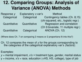
12. Comparing Groups: Analysis of Variance (ANOVA) Methods. Response y Explanatory x var’s Method Categorical Categorical Contingency tables (Ch. 8,15) (chi-squared, etc., logistic regr.)

12. Comparing Groups: Analysis of Variance (ANOVA) Methods
E N D
Presentation Transcript
12. Comparing Groups: Analysis of Variance (ANOVA) Methods Response y Explanatory x var’s Method Categorical Categorical Contingency tables (Ch. 8,15) (chi-squared, etc., logistic regr.) Quantitative Quantitative Regression and correlation (Ch 9 bivariate, 11 multiple regr.) Quantitative Categorical ANOVA (Ch. 12) (Where does Ch. 7 on comparing 2 means or 2 proportions fit into this?) Ch. 12 compares the mean of y for the groups corresponding to the categories of the categorical explanatory var’s (factors). Examples: y = mental impairment, x’s = treatment type, gender, marital status y = income, x’s = race, education (<HS, HS, college), type of job
Comparing means across categories of one classification (1-way ANOVA) • Let g = number of groups • We’re interested in inference about the population means m1 , m2 , ... , mg • The analysis of variance (ANOVA) is an F test of H0: m1 = m2 = = mg Ha: The means are not all identical • The test analyzes whether the differences observed among the sample means could have reasonably occurred by chance, if H0 were true (due to R. A. Fisher).
One-way analysis of variance • Assumptions for the F significance test : • The g population dist’s for the response variable are normal • The population standard dev’s are equal for the g groups (s) • Randomization, such that samples from the g populations can be treated as independent random samples (separate methods used for dependent samples)
Variability between and within groups • (Picture of two possible cases for comparing means of 3 groups; which gives more evidence against H0?) • The F test statistic is large (and P-value is small) if variability between groups is large relative to variability within groups • Both estimates unbiased when H0 is true (then F tends to fluctuate around 1 according to F dist.) • Between-groups estimate tends to overestimate variance when H0 false (then F is large, P-value = right-tail prob. small)
Detailed formulas later, but basically • Each estimate is a ratio of a sum of squares (SS) divided by a df value, giving a mean square (MS). • The F test statistic is a ratio of the mean squares. • P-value = right-tail probability from F distribution (almost always the case for F and chi-squared tests). • Software reports an “ANOVA table” that reports the SS values, df values, MS values, F test statistic, P-value. (Looks like ANOVA table for regression.)
Exercise 12.12: Does number of good friends depend on happiness? (GSS data) Very happy Pretty happy Not too happy Mean 10.4 7.4 8.3 Std. dev. 17.8 13.6 15.6 n 276 468 87 Do you think the population distributions are normal? A different measure of location, such as the median, may be more relevant. Keeping this in mind, we use these data to illustrate one-way ANOVA.
ANOVA table Sum of Mean Source squares df square F Sig Between-groups 1627 2 813 3.47 0.032 Within-groups 193901 828 234 Total 195528 830 The mean squares are 1627/2 = 813 and 193901/828 = 234. The F test statistic is the ratio of mean squares, 813/234 = 3.47 If H0 true, F test statistic has the F dist with df1 = 2, df2 = 828, and P(F ≥ 3.47) = 0.032. There is quite strong evidence that the population means differ for at least two of the three groups.
Within-groups estimate of variance • g = number of groups • Sample sizes n1 ,n2 , … , ng ,, N = n1 + n2 + … + ng • This pools the g separate sample variance estimates into a single estimate that is unbiased, regardless of whether H0 is true. (With equal n’s, s2 is simple average of sample var’s.) • The denominator, N – g, is df2 for the F test.
For the example, this is which is a mean square error (MSE). Its square root, s = 15.3, is the pooled standard deviation estimate that summarizes the separate sample standard deviations of 17.8, 13.6, 15.6 into a single estimate. (Analogous “pooled estimate” used for two-sample comparisons in Chapter 7 that assumed equal variance.) Its df value is (276 + 468 + 87) – 3 = 828. This is df2 for F test, because the estimate s2 is in denominator of F statistic.
Between-groups estimate of variancewhere is the sample mean for the combined samples. (Can motivate using variance formula for sample means, as described in Exercise 12.57.)Since this describes variability among g groups, its df = g – 1, which is df1 for the F test (since between-groups estimate goes in numerator of F test statistic). For the example, between-groups estimate = 813, with df = 2, which is df1 for the F test.
Some commentsabout the ANOVA F test • F test is robust to violations of normal population assumption, especially as sample sizes grow (CLT) • F test is robust to violations of assumption of equal population standard deviations, especially when sample sizes are similar • When sample sizes small and population distributions may be far from normal, can use the Kruskal-Wallis test, a nonparametric method. • Can implement with software such as SPSS (next) • Why use F test instead of several t tests?
Doing a 1-way ANOVA with software • Example: Data in Exercise 12.6. You have to do something similar on HW in 12.8(c). Quiz scores in a beginning French course Mean Standard deviation Group A: 4, 6, 8 6.0 2.0 Group B: 1, 5 3.0 2.8 Group C: 9, 10, 5 8.0 2.6 Report hypotheses, test stat, df values, P-value, interpret
ANOVA table Sum of Mean Source squares df square F Sig Between-groups 30.0 2 15.0 2.5 0.177 Within-groups 30.0 5 6.0 Total 60.0 7 If H0: m1 = m2= m3 were true, probability would equal 0.177 of getting F test statistic value of 2.5 or larger. This is not much evidence against the null. It is plausible that the population means are identical. (But, not much power with such small sample sizes)
Follow-up Comparisons of Pairs of Means • A CI for the difference (µi -µj) is where t-score is based on chosen confidence level, df = N – g for t-scoreis df2 for F test, and s is square root of MSE (within-groups estimate from ANOVA table). Example: A 95% CI for difference between population mean number of close friends for those who are very happy and not too happy is (taking s = 15.3)
(very happy, pretty happy): 3.0 ± 2.3 • (not too happy, pretty happy): 0.9 ± 3.5 The only pair of groups for whom we can conclude the population mean number of friends differ is “very happy” and “pretty happy”. i.e., this conclusion corresponds to the summary: µPH µNTH µVH ________ _________ (note lack of “transitivity” when dealing in probabilistic comparisons)
Comments about comparing pairs of means • In designed experiments, often n1 = n2 = … = ng = n (say), and then the margin of error for each comparison is For each comparison, the CI comparing the two means does not contain 0 if That margin of error called the “least significant difference” (LSD)
If g is large, the number of pairwise comparisons, which is g(g-1)/2, is large. The probability may be unacceptably large that at least one of the CI’s is in error. Example: For g = 10, there are 45comparisons. With 95% CIs, just by chance we expect about 45(0.05) = 2.25 of the CI’s to fail to contain the true difference between population means. (Similar situation in any statistical analysis making lots of inferences, such as conducting all the t tests for parameters in a multiple regression model with a large number of predictors)
Multiple Comparisons of Groups • Goal: Obtain confidence intervals for all pairs of group mean difference, with fixed probability that entire set of CI’s is correct. • One solution: Construct each individual CI with a higher confidence coefficient, so that they will all be correct with at least 95% confidence. • The Bonferroni approach does this by dividing the overall desired error rate by the number of comparisons to get error rate for each comparison.
Example: With g = 3 groups, suppose we want the “multiple comparison error rate” to be 0.05. i.e., we want 95% confidence that all three CI’s contain true differences between population means, 0.05 = probability that at least one CI is in error. • Take 0.05/3 = 0.0167 as error rate for each CI. • Use t = 2.39 instead of t = 1.96 (large N, df) • Each separate CI has form of 98.33% CI instead of 95% CI. Since 2.39/1.96 = 1.22, the margins of error are about 22% larger • (very happy, not too happy): 2.1 ± 4.5 • (very happy, pretty happy): 3.0 ± 2.8 • (not too happy, pretty happy): 0.9 ± 4.3
Comments about Bonferroni method • Based on Bonferroni’s probability inequality: For events E1 , E2 , E3 , … P(at least one event occurs) ≤ P(E1 ) + P(E2 ) + P(E3 ) + … Example: Ei = event that ith CI is in error, i = 1, 2, 3. With three 98.67% CI’s, P(at least one CI in error) ≤ 0.0167 + 0.0167 + 0.0167 = 0.05 • Software also provides other methods, such as Tukey multiple comparison method, which is more complex but gives slightly shorter CIs than Bonferroni.
Regression Approach To ANOVA • Dummy (indicator) variable: Equals 1 if observation from a particular group, 0 if not. • With g groups, we create g - 1 dummy variables: e.g., for g = 3, z1 = 1 if observation from group 1, 0 otherwise z2 = 1 if observation from group 2, 0 otherwise • Subjects in last group have all dummy var’s = 0 • Regression model: E(y) = a + b1z1 + b2z2 • Mean for group 1: m1 = a + b1 group 2:m2 = a + b2 • Mean for group 3: m3 = a • Regression coefficientsb1 = m1 – m3and b2 = m2 – m3compare each mean to mean for last group
Example: Model E(y) = a + b1z1+ b2z2 where y = reported number of close friends z1 = 1 if very happy, 0 otherwise (group 1, mean 10.4) z2 = 1 if pretty happy, 0 otherwise (group 2, mean 7.4) z1 = z2 = 0 if not too happy (group 3, mean 8.3) The prediction equation is = 8.3 + 2.1z1 - 0.9z2 Which gives predicted means Group 1 (very happy): 8.3 + 2.1(1) - 0.9(0) = 10.4 Group 2 (pretty happy): 8.3 + 2.1(0)- 0.9(1) = 7.4 Group 3 (not too happy): 8.3 + 2.1(0)- 0.9(0) = 8.3
Test Comparison (ANOVA, regression) m1 = a+ b1 m2 = a+ b2 m3 = a • 1-way ANOVA: H0: m1= m2 =m3 • Regression approach: Testing H0: b1 = b2 = 0 gives the ANOVA F test (same df values, P-value) • F test statistic from regression (H0: b1 = b2 = 0) is F = (MS for regression)/MSE
Regression ANOVA table: Sum of Mean Source Squares df square F Sig Regression 1627 2 813 3.47 0.032 Residual 193901 828 234 Total 195528 830 The ANOVA “between-groups SS” is the “regression SS” The ANOVA “within-groups SS” is the “residual SS” (SSE) • Regression t tests: Test whether means for groups 1 and 2 are significantly different from group 3: H0: b1 = 0 corresponds to H0: m1 – m3 = 0 H0: b2 = 0 corresponds to H0: m2 – m3 = 0
Let’s use SPSS to do regression for data in Exercise 12.6 • Predicted quiz score = 8.0 - 2.0z1 – 5.0z2 • Recall sample means were 6, 3, 8 for groups 1, 2, 3, which this prediction equation generates. • Note regression F = 2.5, P-value = 0.177 is same as before (p. 13 of notes) with 1-way ANOVA
Why use regression to perform ANOVA? • Unify various methods as special case of one analysis e.g. even methods of Chapter 7 for comparing two means can be viewed as special case of regression with a single dummy variable as indicator for group E(Y) = a + bz with z=1 in group 1, z=0 in group 2 so E(Y) = a + b in group 1, E(Y) = a in group 2, difference between population means = b • Being able to handle categorical variables in a regression model gives us a way to model several predictors that may be categorical or (more commonly, in practice) a mixture of categorical and quantitative.
Two-way ANOVA • Analyzes relationship between quantitative response y and two categorical explanatory factors. Example (Exercise 7.50):A sample of college students were rated by a panel on their physical attractiveness. Response equals number of dates in past 3 months for students rated in top or bottom quartile of attractiveness, for females and males. (Journal of Personality and Social Psychology, 1995)
Summary of data: Means(standard dev., n) Gender Attractiveness Men Women More 9.7 (s =10.0, n = 35) 17.8 (s = 14.2, n = 33) Less 9.9 (s = 12.6, n = 36) 10.4 (s = 16.6, n = 27) We consider first the various hypotheses and significance tests for two-way ANOVA, and then see how it is a special case of a regression analysis.
“Main Effect” Hypotheses • A main effect hypothesis states that the means are equal across levels of one factor, within levels of the other factor. H0 : no effect of gender, H0 : no effect of attractiveness Example of population means for number of dates in past 3 months satisfying these are: 1. No gender effect 2. No attractiveness effect Gender Gender Attractiveness Men Women Men Women More 14.0 14.0 10.0 14.0 Less 10.0 10.0 10.0 14.0
ANOVA tests about main effects • Same assumptions as 1-way ANOVA (randomization, normal population dist’s with equal standard deviations in each “group” which is a “cell” in the table) • There is an F statistic for testing each main effect (some details on next page, but we’ll skip this). • Estimating sizes of effects more naturally done by viewing as a regression model (later) • But, testing for main effects only makes sense if there is not strong evidence of interaction between the factors in their effects on the response variable.
Tests about main effects continued (but we skip today) • The test statistic for a factor main effect has form F = (MS for factor)/(MS error), a ratio of variance estimates such that the numerator tends to inflate (F tends to be large) when H0 false. • s = square root of MSE in denominator of F is estimate of population standard deviation for each group • df1 for F statistic is (no. categories for factor – 1). (This is number of parameters that are coefficients of dummy variables in the regression model corresponding to 2-way ANOVA.)
Interaction in two-way ANOVA Testing main effects only sensible if there is “no interaction”; i.e., effect of each factor is the same at each category for the other factor. Example of population means 1. satisfying no interaction 2. showing interaction Gender Gender Attractiveness Men Women Men Women More 12.0 14.0 12.0 14.0 Less 9.0 11.0 9.0 6.0 (see graph and “parallelism” representing lack of interaction) We can test H0 : no interaction with F = (interaction MS)/(MS error) Should do so before considering main effects tests
What do the sample means suggest? Gender Attractiveness Men Women More 9.7 17.8 Less 9.9 10.4 This suggests interaction, with cell means being approx. equal except for more attractive women (higher), but authors report “none of the effects was significant, due to the large within-groups variance” (data probably also highly skewed to right).
An example for which we have the raw data: Student survey data file • y = number of weekly hours engaged in sports and other physical exercise. • Factors: gender, whether a vegetarian (both categorical, so two-way ANOVA relevant) • We use SPSS with survey.sav data file • On Analyze menu, recall Compare means option has 1-way ANOVA as a further option • Something weird in SPSS: levels of factor must be coded numerically, even though treated as nominal variables in the analysis! For gender, I created a dummy variable g for gender For vegetarian, I created a dummy variable v for vegetarianism
Sample means on sports by factor: Gender: 4.4 females (n = 31), 6.6 males (n = 29) Vegetarianism: 4.0 yes (n = 9), 5.75 no (n = 51) • One-way ANOVA comparing mean on sports by gender has F = 5.2, P-value = 0.03. • One-way ANOVA comparing mean on sports by whether a vegetarian has F = 1.57, P-value = 0.22. These are merely squares of t statistic from Chapter 7 for comparing two means assuming equal variability (df for t is n1 + n2 – 2 = 58 = df2 for F test, df1 = 1)
One-way ANOVA’s handle only one factor at a time, give no information about possible interaction, how effects of one factor may change according to level of other factor Sample means Vegetarian Men Women Yes 3.0 (n = 3) 4.5 (n = 6) No 7.0 (n = 26) 4.4 (n = 25) Seems to show interaction, but some cell n’s are very small and standard errors of these means are large (e.g., SPSS reports se = 2.1 for sample mean of 3.0) • In SPSS, to do two-way ANOVA, on Analyze menu choose General Linear Model option and Univariate suboption, declaring factors as fixed (I remind myself by looking at Appendix p. 552 in my SMSS textbook).
Two-way ANOVA Summary General Notation: Factor A has a levels, B has b levels • Procedure: • Test H0: No interaction based on the FAB statistic • If the interaction test is not significant, test for Factor A and B effects based on the FA and FB statistics (and can remove interaction terms from model)
Test of H0 : no interaction has F = 29.6/13.7 = 2.16, df1 = 1, df2 = 56, P-value = 0.15
Since interaction is not significant, we can take it out of model and re-do analysis using only main effects. (In SPSS, click on Model to build customized model containing main effects but no interaction term) • At 0.05 level, gender is significant (P-value = 0.037) but vegetarianism is not (P-value = 0.32)
More informative to estimate sizes of effects using regression model with dummy variables g for gender (1=female, 0=male), v for vegetarian (1=no, 0=yes). • Model E(y) = a + b1g + b2v • Model satisfies lack of interaction • To allow interaction, we add b3(v*g) to model
Predicted weekly hours in sports = 5.4 – 2.1g + 1.4v • The estimated means are: 5.4 for male vegetarians (g = 0, v = 0) 5.4 – 2.1 = 3.3 for female vegetarians (g = 1, v = 0) 5.4 + 1.4 = 6.8 for male nonvegetarians (g=0, v =1) 5.4 – 2.1 + 1.4 = 4.7 for female nonveg. (g=1, v=1) These “smooth” the sample means and display no interaction (recall mean = 3.0 for male vegetarians had only n = 3). Sample means Model predicted means Vegetarian Men Women Men Women Yes 3.0 4.5 5.4 3.3 No 7.0 4.4 6.8 4.7
The “no interaction” model provides estimates of main effects and CI’s • Estimated vegetarian effect (comparing mean sports for nonveg. and veg.), controlling for gender, is 1.4. • Estimated gender effect (comparing mean sports for females and males), controlling for whether a vegetarian, is -2.1. • Controlling for whether a vegetarian, a 95% CI for the difference between mean weekly time on sports for males and for females is 2.077 ± 2.00(0.974), or (0.13, 4.03) (Note 2.00 is t score for df = 57 = 60 - 3)
Comments about two-way ANOVA • If interaction terms needed in model, need to compare means (e.g., with CI) for levels of one factor separately at each level of other factor • Testing a term in the model corresponds to a comparison of two regression models, with and without the term. The SS for the term is the difference between SSE without and with the term (i.e., the variability explained by that term, adjusting for whatever else is in the model). This is called a partial SS or a Type III SS in some software
The squares of the t statistics shown in the table of parameter estimates are the F statistics for the main effects (Each factor has only two categories and one parameter, so df1 = 1 in F test) • When cell n’s are identical, as in many designed experiments, the model SS for model with factors A and B and their interaction partitions exactly into Model SS = SSA + SSB + SSAxB and SSA and SSB are same as in one-way ANOVAs or in two-way ANOVA without interaction term. (Then not necessary to delete interaction terms from model before testing main effects) • When cell n’s are not identical, estimated difference in means between two levels of a factor in two-way ANOVA need not be same as in one-way ANOVA (e.g., see our example, where vegetarianism effect is 1.75 in one-way ANOVA where gender ignored, 1.4 in two-way ANOVA where gender is controlled) • Two-way ANOVA extends to three-way ANOVA and, generally, factorial ANOVA.
For dependent samples (e.g., “repeated measures” over time), there are alternative ANOVA methods that account for the dependence (Sections 12.6, 12.7). Likewise, the regression model for ANOVA extends to models for dependent samples. • The model can explicitly include a term for each subject. E.g., for a crossover study with t = treatment (1, 0 dummy var.) and pi = 1 for subject i and pi = 0 otherwise, assuming no interaction, E(y) = a + b1p1+ b2 p2 + … + bn-1pn-1 + bnt • The number of “person effects” can be huge. Those effects are usually treated as “random effects” (random variables, with some distribution, such as normal) rather than “fixed effects” (parameters). The main interest is usually in the fixed effects.
In making many inferences (e.g., CI’s for each pair of levels of a factor), multiple comparison methods (e.g., Bonferroni, Tukey) can control overall error rate. • Regression model for ANOVA extends to models having both categorical and quantitative explanatory variables (Chapter 13) Example: Modeling y = number of close friends, with predictors g =gender (g = 1, female, g = 0 male), race (r1 = 1, black, 0 other; r2 = 1, Hispanic, 0 other, r1 = r2 = 0, white) x1 = number of social organizations a member of x2 = age Model E(y) = a + b1g+ b2 r1 + b3r2 + b4 x1 + b5 x2
How do we do regression when response variable is categorical (Ch. 15)? • Model the probability for a category of the response variable. E.g., with binary response (y = 1 or 0), model P(y = 1)in terms of explanatory variables. • Need a mathematical formula more complex than a straight line, to keep predicted probabilities between 0 and 1 • Logistic regression uses an S-shaped curve that goes from 0 up to 1 or from 1 down to 0 as a predictor x changes
Logistic regression model • With binary response (y = 1 or 0) and a single explanatory variable, model has form • Then the odds satisfies (exponential function) and odds multiplies by e for each 1-unit increase in x; i.e., e is an odds ratio i.e., the odds for y = 1instead of y = 0at x+1 divided by odds at x.
For this model, taking the log of the odds yields a linear equation in x, • The log of the odds is called the “logit,” and this type of model is sometimes called a logit model. • This logistic regression model extends to many predictors
As in ordinary regression, it’s possible to have quantitative and categorical explanatory variables (using dummy variables for categorical ones). • Example: For sample of elderly, y = whether show symptoms of Alzheimer’s disease (1 = yes, 0 = no) • x1 = score on test of mental acuity • x2 = physically mobile (1 = yes, 0 = no) A model without an interaction term implies “parallel S-shaped curves” when fix one predictor, consider effect of other predictor A model with interaction implies curves have different rate of change (picture)