Download
1 / 17
170 likes | 665 Vues
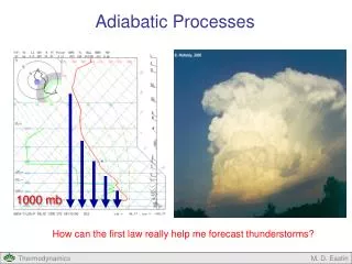
ATMOSPHERIC PROCESSES--PSEUDOADIABATIC Adiabatic wet-bulb temperature Adiabatic equivalent temperature Conservative properties. Reversible Saturated Adiabatic Processes If we consider a closed parcel of rising, cloudy air, the process is reversible since all the

E N D
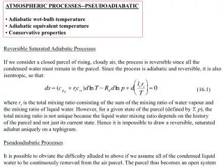
ATMOSPHERIC PROCESSES--PSEUDOADIABATIC • Adiabatic wet-bulb temperature • Adiabatic equivalent temperature • Conservative properties Reversible Saturated Adiabatic Processes If we consider a closed parcel of rising, cloudy air, the process is reversible since all the condensed water must remain in the parcel. Since the process is adiabatic and reversible, it is also isentropic, so that: (16.1) where rtis the total mixing ratio consisting of the sum of the mixing ratio of water vapour and the mixing ratio of liquid water. However, for a given state of the parcel (defined by T, p), the total mixing ratio is not unique because the liquid water mixing ratio depends on the history of the parcel and not just its current state. Hence it is impossible to draw a reversible, saturated adiabat uniquely on a tephigram. Pseudoadiabatic Processes It is possible to obviate the difficulty alluded to above if we assume all of the condensed liquid water to be continuously removed from the air parcel. The parcel thus becomes an open system
and the process is irreversible. However, if we assume that the process can be divided into an infinite sequence of infinitesimal two-stage processes (see Note below), we may write for the pseudo-adiabatic process: (16.2) [Note: These two-stage processes are an infinitesimal reversible saturated adiabatic expansion and condensation, followed by the removal of an infinitesimal amount of condensed liquid water, without changing T, p.] Despite the theoretical differences between Eq. 16.1 and 16.2 (i.e., using the saturation mixing ratio in 16.2 as opposed to the total mixing ratio in 16.1), the practical difference is small. Hence an approximation to both the saturated adiabatic and pseudoadiabatic processes is given by: (16.3) Integration of Eq. 16.3 leads to the pseudoadiabats on the tephigram (the zebra-stripe curves). Adiabatic Wet-Bulb Temperature, Taw The adiabatic wet-bulb temperature is defined by the following process on a tephigram:
1. Starting at (T,p,r), follow a moist adiabat upwards (actually a dry adiabat) to the saturation point (the point at which the adiabat intersects the equisaturated curve with rs=r). This point is also known as the lifting condensation level (LCL). 2. From the LCL, descend along a pseudoadiabat to the original pressure, p. 3. The temperature at this point is the adiabatic wet-bulb temperature. Note that the result of this process is that the original air parcel is now saturated and at the initial pressure. Its temperature, however, has dropped because of the heat which was required to evaporate liquid water into it (which had to be derived from its internal energy since the process was adiabatic). The final state of the parcel is therefore similar to that which occurs during adiabatic, isobaric evaporation of liquid water, leading to the isobaric wet-bulb temperature. However, the adiabatic wet-bulb temperature and the isobaric wet-bulb temperature are not identical. The explanation is a simple one. In reaching the isobaric wet-bulb temperature, the liquid water is evaporated into the parcel at temperatures higher than Tiw. But in reaching the adiabatic wet-bulb temperature, the liquid water is evaporated into the parcel at temperatures lower than Taw. Since the specific latent heat of vapourization decreases with temperature, there is less latent heat required to evaporate the same mass of liquid water isobarically than there is adiabatically. As a result, Tiw > Taw, although the difference is generally only a fraction of a degree. See the sketch below for an illustration of these two processes.
Adiabatic Equivalent Temperature, Tae The adiabatic equivalent temperature is defined by the following processes on the tephigram: Starting at (T,p,r), ascend along a dry adiabat to the LCL. Continue to ascend along a pseudoadiabat from the LCL, until the air parcel is dry (practically speaking, you can only go as far as the -50oC isotherm). Descend along a dry adiabat to the original pressure. The temperature at this point is the adiabatic equivalent temperature. The outcome of this process is a dry air parcel at the initial pressure. Its temperature is higher than the initial temperature because of the release of the latent heat of condensation. The final state is thus similar to the final state defined by the isobaric equivalent temperature (although
the process required to achieve the latter is impossible, while the process required to achieve the adiabatic equivalent temperature is possible, at least in principle). The condensation in the process leading to the adiabatic equivalent temperature occurs at temperatures below the saturation temperature, while the condensation in the process leading to the isobaric equivalent temperature occurs at temperatures above the initial temperature. Because the specific latent heat of condensation decreases with temperature, there is more latent heat released in the adiabatic process than in the isobaric process. Consequently, Tae>Tie, and the difference can be several degrees. The adiabatic wet-bulb potential temperature, aw, can be found by simply continuing down the pseudoadiabat to 100 kPa and reading the temperature there. Similarly, the adiabatic equivalent potential temperature, ae, can be found by continuing down the final dry adiabat to 100 kPa and reading the temperature there. (See the previous diagram.)
CONSERVATIVE PROPERTIES The table below indicates which thermodynamic properties are conserved (denoted by “C”) and which are not conserved (denoted by “N”) under various atmospheric processes. The conservative properties are particularly valuable in helping to identify and track air masses.
THE HYDROSTATIC EQUATION • Geopotential energy • Hydrostatic equation Geopotential Energy A scale analysis of the vertical equation of motion leads to a very convincing near-equilibrium between the vertical pressure gradient force and the force of gravity: (17.1) Note that if we consider only the vertical direction then we would have For those of you who are not students of dynamical meteorology, this equation can be readily derived by considering the balance of forces acting on an air parcel of height dz in a column of unit cross-sectional area, as in the figure below:
Because gravity is a conservative force (i.e., one for which ), it can be defined as the gradient of a potential function: (17.2) You should verify for yourself that if then gravity is a conservative force. Therefore, surfaces of constant potential function, , are perpendicular to gravity and vice versa. Thus we see that is the potential energy per unit mass required to lift an air parcel from mean sea level (our chosen reference height) to a certain height, z. (Recall that work, or energy, equals force times distance so that for a unit mass, Eq. 17.2 is just such a statement.) (17.3) We can now use to define a new height scale. Let: (17.4) where g0=9.80665m/s2 is the acceleration due to gravity at mean sea level. Z is the height in geopotential metres. The chief advantage of using Z rather than the geometric height, z, is that we can consider the acceleration due to gravity to be a constant when integrating, since:
(17.5) Having made the distinction between the geopotential height and geometrical height, we will now drop the adjective. Although the numerical difference between the two is only about 0.1% or less in the troposphere, ignoring the difference could mean ignoring a significant amount of potential energy. Even a 10 metre height discrepancy corresponds to an error in potential energy that could convert into a wind error of almost 15 m/s (use 0.5v2=g0Z). Consequently, geopotential height is an important concept, and when the term height is used by a meteorologist, it is safe to assume that geopotential height is what is meant. The table below shows a comparison between geometric height and geopotential height (both measured from mean sea level) at 40oN.
MODEL ATMOSPHERES • Model atmospheres • Rawinsonde height computations • Reduction of pressure to sea level Model Atmospheres We will consider here four idealized atmospheres and examine the lapse rates of pressure, density, and temperature within them. Each of these atmospheres is a suitable model of the real atmosphere (or a portion of it), under certain circumstances (you should try to figure out what these are). HOMOGENEOUS ATMOSPHERE (=constant) A homogeneous atmosphere is one with constant density. Because the real atmosphere is compressible, it cannot be homogeneous. By contrast, the ocean is approximately homogeneous because its compressibility is about 10-4 times that of air. If we consider an atmospheric layer of thickness 100 m, the variation of density across it is only about 1%. Hence, such a layer (or a thinner one) could be considered to be approximately homogeneous. Ignoring this caveat, if we were to consider the entire atmosphere to be homogeneous, it would have to have a finite thickness (unlike the real atmosphere). This thickness, H, can be determined by integrating the hydrostatic equation 17.1:
(18.1) where the subscript “0” denotes mean sea level conditions, and the final equation is obtained by making use of the ideal gas law. Using appropriate values leads to a value of H~8 km. H is known as the scale height. The temperature lapse rate in a homogeneous atmosphere can be deduced by equating the vertical pressure gradient expressions from the ideal gas law and the hydrostatic equation (17.1): (18.2) from which the lapse rate, -dT/dz, is given by: =g/R~34 K/km. You may recall that this is the autoconvective lapse rate. That is, if the temperature diminished even more rapidly with height than this value, the density would begin to increase with height and the result would clearly be convectively unstable. It is possible to get such high lapse rates (or even higher ones) very close (i.e., within a few centimetres) to a sun-warmed surface. Even over the distance of our bodies, lapse rates can be generally quite large over a hot surface such as a road. In such cases, even though the atmosphere tries valiantly to vertically redistribute the surface heat by convective overturning, the resulting rate of heat transfer is not great enough to overcome the effects of the solar heating. Hence it is possible, very near a hot surface, to have a density profile which increases with height. This can lead to refraction of light in the atmosphere in such a way as to
give rise to the so-called superior mirage (e.g., apparent pools of water on a hot surface, as in the diagram below). You can also see this effect above large campfires during the day (as well as the effect of temperature on sound speed if you listen carefully to the people across the fire from you!). 2. ISOTHERMAL ATMOSPHERE (T=constant) We shall show that, in an isothermal atmosphere, the pressure and density decrease exponentially with height, and that the e-folding height (the height at which pressure or density is a factor of 1/e times its value at the surface) is equal to the scale height. We begin by substituting the ideal gas law into the hydrostatic equation and integrating: (18.3) The exponential decrease of density with height follows readily from Eq. 18.3 and the ideal gas law for constant temperature.
By definition, the temperature lapse rate is zero in an isothermal atmosphere. In the real atmosphere, the pressure decreases approximately exponentially with height, with a scale height of about 7.3 km. Although the real atmosphere is not isothermal, the variation in absolute temperature is only about 20% over the region of meteorological interest (the troposphere and the stratosphere), with the result that an isothermal approximation is “not bad” (at least for some purposes). A more useful number, however, is the half-height of the atmosphere, which is about 5 km. This means that the pressure falls by a factor of about 2 for every 5 km increase in height. 3. CONSTANT LAPSE RATE ATMOSPHERE A constant lapse rate atmosphere is one in which the temperature varies linearly with height: (18.4) with a constant. If the temperature sounding in the real atmosphere can be approximated by a piecewise-linear function (i.e., a sequence of straight lines), then a constant lapse rate model can be applied to each of these linear layers. Integrating the hydrostatic equation gives: (18.5)
Like the homogeneous atmosphere, a constant lapse rate atmosphere has a finite height. At the top, T=0, p=0, and this implies a thickness of T0/. Since Eq. 18.5 should be valid for all lapse rates, we can ask the question: what is the result when 0? Recalling that we can manipulate Eq. 18.5 as follows: as for an isothermal atmosphere. 4. DRY ADIABATIC ATMOSPHERE A dry adiabatic atmosphere is a special case of a constant lapse rate atmosphere, and has: (18.6) 5. U.S. STANDARD ATMOSPHERE The U.S. Standard Atmosphere is an atmospheric model created by a committee in 1962. It is supposed to represent the annual average characteristics of the real atmosphere in mid-latitudes
(40N) up to an altitude of 32 km. It consists of a sequence of constant lapse rate layers, as in the diagram below: RAWINSONDE HEIGHT COMPUTATIONS Rawinsonde balloons generally measure T, p, Td at regular intervals (~10s) as they ascend at a speed of about 5 m/s. This gives roughly 50 m resolution in the vertical, or 5 mb near the surface. In order to determine the local height of isobaric surfaces (the height field on an isobaric surface determines the geostrophic wind field, and hence is a very essential meteorological variable) the sounding data can be integrated using the hydrostatic equation. This is done as follows. First, Td is used to determine the mixing ratio r=rs(Td). Then we determine the specific humidity from q=r/(1+r), and then the virtual temperature from Tv=T(1+0.87q). Then, beginning with the hydrostatic equation (17.1) but now taking z to be the geopotential height, and hence g=g0, the
constant mean sea-level value. Substituting from the ideal gas law for moist air in the form p=RdTv, we can integrate the hydrostatic equation to yield: (18.8) where z2-z1 is known as the thickness between the pressure levels p1and p2. The geopotential height at the surface can be determined once and for all for each rawinsonde station. Thereafter, Eq. 18.8 can be integrated from the surface numerically. Alternatively, one may use the tephigram to obtain the mean temperature over a finite pressure interval, as in the sketch below. Using this mean temperature, the thickness between significant pressure levels can then be looked up on the tephigram. Alternatively, on may use the mean value theorem to evaluate Eq. 18.8, giving: (18.9)
REDUCTION OF PRESSURE TO MEAN SEA LEVEL Surface weather charts depict isobars on a zero-height surface (mean sea level). However, not all observing stations are at sea level, so the observed station pressure must be adjusted (normally, this means increased) to mean sea level. If one did not do this, there would be permanent low pressure areas over mountainous and hilly terrain, which would make it difficult to identify the transient cyclonic systems which are associated with weather. In order to perform the necessary adjustment, we imagine that a hole is drilled in the ground (with a cross-section of 1 square metre) down to mean sea level. Then we increment the measured station pressure by the weight of the air in the hole. Equivalently, inverting Eq. 18.9, we have: (18.10) where p2 is the measured station pressure, z2 is the geopotential height of the rawinsonde station, and is the mean virtual temperature of the air in the hole. The problem is that there is no hole, and hence no way to measure this mean virtual temperature. So we suppose, for this purpose, that the temperature at the top of the hole is the average of the current station temperature and the temperature twelve hours ago, and that the lapse rate in the hole is 5o C/km.