Forecasting Introduction

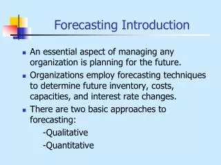
1. Forecasting Introduction • An essential aspect of managing any organization is planning for the future. • Organizations employ forecasting techniques to determine future inventory, costs, capacities, and interest rate changes. • There are two basic approaches to forecasting: -Qualitative -Quantitative

2. Long-range time spans usually greater than one year necessary to support strategic decisions about planning products, processes, and facilities Short-range time spans ranging from a few days to a few weeks cycles, seasonality, and trend may have little effect random fluctuation is main data pattern Time Span of Forecasts

3. Qualitative Approaches to Forecasting • Delphi Approach • A panel of experts, each of whom is physically separated from the others and is anonymous, is asked to respond to a sequential series of questionnaires. • Scenario Writing • Subjective or Interactive Approaches

4. Quantitative Approaches to Forecasting • Quantitative methods are based on an analysis of historical data concerning one or more time series. • A time series is a set of observations measured at successive points in time or over successive periods of time. • If the historical data used are restricted to past values of the series that we are trying to forecast, the procedure is called a time series method. • If the historical data used involve other time series that are believed to be related to the time series that we are trying to forecast, the procedure is called a causal method.

5. Trendsaccounts for the gradual shifting of the time series over a long period of time. Seasonalityof the series accounts for regular patterns of variability within certain time periods, such as over a year. CycleAny regular pattern of sequences of values above and below the trend line is attributable Random fluctuationseries is caused by short-term, unanticipated and non-recurring factors that affect the values of the time series. Time series data-Data Patterns

6. Smoothing Methods: Moving Average • Moving Average Method The moving average method consists of computing an average of the most recent n data values for the series and using this average for forecasting the value of the time series for the next period. • Error in Forecasting • Measures the average error that can be expected over time.

7. Moving Averages

8. Moving Averages Forecast

9. This is a variation on the simple moving average where instead of the weights used to compute the average being equal, they are not equal This allows more recent demand data to have a greater effect on the moving average, therefore the forecast The weights must add to 1.0 and generally decrease in value with the age of the data The distribution of the weights determine impulse response of the forecast Weighted Moving Average = w1Yt + w2Yt-1 +w3Yt-2 + …+ wnYt-n+1 Swi = 1

10. Weighted Moving Average

11. Weighted Moving Average

12. Moving Average - Example

13. Vacuum cleaner sales for 12 months is given below. The owner of the supermarket decides to forecast sales by weighting the past 3 months as follows Weighted Moving Average

14. The weights used to compute the forecast (moving average) are exponentially distributed The forecast is the sum of the old forecast and a portion of the forecast error Ft = Ft-1 + a(At-1-Ft-1) The smoothing constant, , must be between 0.0 and 1.0 A large  provides a high impulse response forecast A small  provides a low impulse response forecast Exponential Smoothing New Forecast = a (Actual Demand) + (1-a)(Old Forecast)

15. Exponential Smoothing Data

16. Exponential Smoothing (Alpha = .42)

17. Estimate the trend values using the data given by taking a 4 yr moving average. In January a city hotel predicted a February demand for 142 room occupancy. Actual February demand was 153 rooms. Using α= .20 forecast the march demand using exponential smoothing method Exponential Smoothing - example