Download
1 / 40
400 likes | 430 Vues
This study evaluates the statewide effects of transportation policy in California by modeling strategies that reduce petroleum dependence. The analysis covers projections for the California economy in 2000, 2020, and 2050 using a comprehensive computable general equilibrium model called EDRAM. By examining different scenarios and factors such as migration data, trade elasticities, and petroleum elasticity between capital and labor, the study aims to understand the economy-wide impacts of reducing petroleum consumption. The model accounts for 102 distinct sectors, including industrial, consumer, government, and household sectors, and simulates outcomes such as fuel efficiency improvements and fuel savings to consumers and industries. Through scenarios like fuel economy improvements, hydrogen fuel adoption, and full hybrid vehicles, the study explores the implications on prices, imports, production, and sensitivity to world oil prices. The findings provide insights into the potential benefits and challenges of transitioning towards more sustainable transportation practices in California.

E N D
Statewide Effects of Transportation Policy By Peter Berck University of California, Berkeley August 2002
The Task: Assembly Bill 2076 • Evaluate the likely economy wide effects of petroleum dependence reducing strategies in the context of projections for the California economy for 2000, 2020 and 2050. • Method: EDRAM, a computable general equilibrium model for the California economy.
DRAM & EDRAM • Models of the entire California Economy. • DRAM is used to evaluate proposal with large fiscal impact. • EDRAM is a derivative model with pollution coefficients and more detail about industrial sectors.
Uncertainty in Model • 1998 base from 1992 IO table • Migration data • Trade elasticities • Petroleum elasticity of subs between capital and labor
General Equilibrium • The model solves for the prices of goods and services and factors of production that make quantity demanded and supplied equal. • Both physical goods and money are conserved.
Structure of E-DRAM • 102 distinct sectors: • 29 industrial sectors, • 9 consumer sectors, • two factor sectors (labor and capital), • seven household sectors, • one investment sector, • 45 government sectors, and • one sector that represents the rest of the world.
Refining Crude Production Import and Export Crude Refined Intermediate good purchased by Transportation Other sectors Purchased by consumers Significant direct tax revenue Engines are needed to use petroleum Where is Petroleum?
Goods and Services 29 different goods and services and 29 types of firms Two Factors: Capital and Labor
Investment and Migration • Immigration and emigration respond to economic conditions. • Investment and disinvestment respond to the rate of return. • Model is equilibrium—takes 3-5 years to fully adjust to policy changes.
Equilibrium • No modeling of transient phenomena • Temporary supply disruptions • Temporary price spikes • Cyclical unemployment and low capacity utilization • Petroleum depletion accounted for only in terms of cost increases for imports
The Base Years • 1998/99. EDRAM with the Petroleum sector modified to correspond to Energy Information Administration numbers and then balanced to produce consistent accounts. • 2020. Matches projections for growth in population and state personal income.
…Base Years • 2050. Growth rates continued from 2020, except California oil production ends and refinery sector does not increase in capacity.
Fuel Efficiency EEA/Duleep Fuel Economy Improvements ACEEE-Advanced Fuel Economy Improvements Fuel Efficiency plus fuel displacement ACEE-Moderate + Fuel Cell Vehicles ACEEE-Full Hybrid Vehicles Four Scenarios
Scenario 1: EEA/Duleep All figures in millions of dollars.
Implementation of Scenario 1 • The price of consumer transportation increases by 90% of $1.961 billion cost. • Price to consumers of transportation (net of fuel ) increases by this fraction: • (Base transp. Expend. + 0.9*1.961)/(base transp. Expenditure)1] • All industrial sectors require more of the ENGIN sector to produce a unit of their output. • Engin requirements increase to require 10% of the $1.96 billion in costs in the base case plus the $.125 billion for diesel. • ENGIN requirements increase by this factor: • (Base expenditure on ENGIN + .1*1.961 + .125)/(base exp. on Engin.)
Implementation… continued • 90% of the $3.264b fuel savings to consumers. • Decreases effective fuel price to consumer by this fraction: • (base fuel expend. - .9*3.264 )/(base fuel expend) • 10% of the $3.264b fuel savings to industry • Every unit of output for every industry requires less fuel input by this fraction • (base fuel expend. - .1*3.264 )/(base fuel expend)
Scenario 2: ACEE-Ad. Fuel All figures in millions of dollars.
Implementation • Same structure as Scenario 1 • Larger vehicle costs • Larger fuel savings
Scenario 3: Fuel Cell + All figures in millions of dollars.
Scenario 3 • Same structure as 1 plus • Additional expenditure for hydrogen fuel • Purchased from the Chemical sector rather than ENMIN • $776 Million in 2020 • $8.7 Billion in 2050 • Applied as before increase in the percent of purchases by PETRO of CHEM • And a percentage decrease by PETRO of ENMIN
Scenario 4: Full Hybrid All figures in millions of dollars.
Implementation of 4 • Scenario 4 has the same economic structure as scenario 1.
Sensitivity to World Price • Increased world price of Petro and Crude increases benefits of scenarios and leaves their costs unchanged. • 20% increase in price in 2020. • Personal income is increased over base in 3 of 4 scenarios and falls less in the fourth. • As price increases, scenarios become clearly preferred to base
Senstivity to Imports • Decreasing the supply elasticity of imports accelerates the decline of the domestic industry. • Conversely, increasing their elasticity moderates that decline. • In the case of ENMIN it approx triples the decline to go from e= 2 to e=.1
Sensitivity to Fuel Price Elas. • If e= -.77 rather than -.2, the effects on state wide aggregates would be dampened. • Scen 4 2020: .2% output fall rather than .5% • Reason: consumers don’t contract their fuel use as much—the lower effective price counters the technical efficiency
Conclusions Consumers: All the scenarios result in much lower effective fuel prices. Prices for transport services are higher. Savings from fuel are spent on other items including apparel and food Consumers whose income is largely wages see an increase in their real incomes; this leads to a larger labor supply
Conclusions cont. • As a result of fuel savings, the petroleum industry contracts in all scenarios, more in those scenarios where more fuel is saved. • Energy minerals contracts for the same reason. • Contraction of these sectors reduces non-wage payments to consumers. • Consumers with a high fraction of income from capital see their real incomes decrease in many scenarios
Conclusions….cont • As a result of these competing forces, personal income is mixed: In 2020 scenarios 1-3 PI changes by roughly the calibration error. In scenario 4 it is down by .4%. • In 2050 personal income is never down by much more than the calibration error and increases in three scenarios.
Conclusions… cont. • State Output falls, because of the contraction of the petroleum sector. In 2020 scenarios between 37% and 57% of the output decrease is directly attributable to the decrease in PETRO. • Labor increases, because laborers are more sensitive to real wages than to returns to capital. • The scenarios range from mild to very aggressive fuel saving scenarios and have only very modest effect upon the economy as a whole. • An increase in oil prices makes all the scenarios more attractive in terms of PI, real wages, and GSP.