Download
1 / 54
540 likes | 665 Vues
Explore tax incidence and equivalence in Harberger General Equilibrium Model with examples and implications of perfect competition. Understand the effects of specific vs. lump-sum taxes on factor supplies and corporate income tax burden.

E N D
Unit 8 Seminar Tax Incidence: Applications Cost Benefit Analysis
The Harberger General Equilibrium Model of Tax Incidence Variation of typical two-goods (X, Y) and two-factors (K,L) general equilibrium model Individuals have identical utility functions over X and Y, goods and factor markets are perfectly competitive, and there are no pure economic profits for firms It must also be assumed that Y is relatively capital-intensive and X is relatively labor-intensive (required to guarantee the prices of the goods and the factors vary as the economy moves from one equilibrium to another along the frontier)
The assumption of perfect competition has two important implications: The capital and labor supplied to the market must always be fully employed in equilibrium If there is unemployment, then production would fall until the X and Y firms are willing to hire all of the labor Individuals have to receive the same wages and same return to capital whether they are used in the production of X or Y If not, then workers would move between X and Y firms, driving up the wages in the firm they left and driving down wages in the firm they entered, until equality was reached Perfect Competition
Tax Incidence Equivalence • Because Harberger assumes that all tax revenues collected are returned lump-sum, it holds that the incidence and the impact of lump-sum taxes are identical • Examples include taxes on individual income earned from labor supply or supply of capital and broad-based tax on Haig-Simons income • Because the side of the market taxed does not matter: • A payroll tax on all firms’ use of labor is equivalent to an income tax on wages received • A tax on all firms’ returns to capitalis equivalent to an income tax on the earnings from capital • A value-added tax on payments to labor and capital by all firms is equivalent to a broad-based income tax
Note: These factor taxes are all lump-sum so if revenue is returned lump-sum, they do not affect prices or factor allocations between X and Y firms (i.e. their incidence and impact is equal) Equivalence between broad-based taxes implies equivalence between an expenditure tax on both goods and a broad-based income tax A general sales tax levied on both the Y and X firms is equivalent to a value-added tax on the payments to labor and capital by both firms None of these taxes has any effect on the economy if the revenues are all returned lump sum to individuals - This means that the only interesting taxes, at least in terms of analyzing tax incidence, are specific taxes that are distorting and notlump sum Tax Incidence Equivalence continued
Harberger assumed that the relatively capital-intensive Y firms were corporations and the relatively labor-intensive X firms were non-corporate businesses The corporate income tax makes K more expensive and raises the marginal cost of producing Y If Y and X are substitutes in consumption, this increases the demand for X - Post-tax prices are assumed to be equal because the tax drives the economy below its production possibility frontier so that the marginal rate of technical substitution are no longer equal for X and Y firms The Incidence of Corporation Income Tax
- Supply of capital is assumed to be fixed The corporate income tax causes the demand for capital by the Y firms to shift down by the full amount of the tax This reduction causes owners of capital to shift from Y to X firms which causes capital supply curves to shift until the net rates of return are equal Result is that all suppliers of capital lose (and government’s desire to impose burden only on corporation stockholders fails) The Incidence of Corporation Income Tax cont’d
In this model, the incidence of the tax depends on: The size of the tax The importance of the taxed factor to the industry being taxed Both determine the degree to which taxed firms react to the tax (i.e. how much the supply curves above move) The elasticities of demand for X and Y Determines the degree to which shifting of resources occurs between X and Y (i.e. how much quantity demanded of Y decreases and demand for X increases) (4) The elasticity of substitution between K and L in the two industries Determines the slope of the demand curves for capital The Incidence of Corporation Income Tax cont’d
Harberger noted that the best empirical estimates of the final three factors, at the time, suggested that the return to capital would fall so far that capital would suffer almost the entire burden of the tax Most economists agree that the burden of the corporate income tax falls almost entirely on the suppliers of capital The Incidence of Corporation Income Tax cont’d
Variable factor supplies Assuming factors of production are variable rather than fixed, results in major taxes are no longer lump-sum This means that the incidence is no longer the impact The biggest difference occurs in the long-run, in an overlapping generations (OLG) model This is because the corporate income tax is borne primarily by the suppliers of capital, the savings rate decreases in the long-run which decreasesinvestment, the marginal product of labor and the real wage (which means that some portion of tax becomes borne by labor) Variations in the Baseline Model
Non-identical individuals Affects individuals in a static context as a tax on good X that raises the relative price ratio, forcing more of the burden onto those who consume a higher proportion of X In an OLG model, a switch from an income to an expenditure tax places a disproportionate burden on the older/retired generation by taxing them for a third time on their working years income. The three taxes are: They saved out of post-tax dollars They paid taxes on the interest earned on savings They now pay expenditure tax as they spend their savings Variations in the Baseline Model continued
Overall then, the supply tax has no effect on the market for capital It does impact local owners of capital though, as the net-of-tax-price decreases by the full amount of the tax so that they suffer the full burden of the tax A capital income tax on firms within the locality (a demand-side tax) shifts the demand curve for capital down by the full amount of the tax Here the equilibrium amount of capital decreases, the price of capital to firms increases, and the return top owners of capital remains the same Variations in the Baseline Model continued
This demonstrates that the tax-on-demand side differs from the tax-on-supply side in two important respects: The demand-side tax does not burden local owners of capital like the supply-side tax does Only the demand-side tax lowers the amount of labor and capital employed in the state or locality and the amount of output produced (i.e. is “anti-business”) Variations in the Baseline Model continued
Harberger argues that under perfect competition the burden of the corporate income tax is borne largely by stockholders Large, price-setting oligopolies are found almost exclusively in the corporate business sector Harberger’s assumption of perfect competition is probably not accurate for effect of corporate income tax in such cases Economists have not settled on a general theory of oligopoly Based on existing theories, it is possible that managers of large corporations can avoid some of the burden of a corporate income tax by exerting their market power If the corporation is initially maximizing market share by producing above profit-maximizing output, stockholders can avoid the burden of the tax by insisting the firm cut back on production and raise prices Non-Competitive Markets
The Sources and Uses Analysis of Incidence Developed by Joseph Pechman of the Brookings Institution Designed to exploit the detailed data sets on individuals and families that various government agencies were collecting and making available to researchers Approach used a variety of assumptions and results in the literature to allocate the burden of the major U.S. taxes to the different sources and uses of income of individuals and families in the databases, before looking at income deciles to determine whether taxes were regressive, proportional, or progressive Sources defined as transfers received and also earned income, consisting of income from labor, capital, and land Usesdefinedas consumption and saving
The allocation of tax burden to sources and uses matters because: Transfers disproportionately go to the poor Income from capital disproportionately goes to the wealthy The ratio of consumption to income falls sharply as income rises Tax burdens allocated to transfers and consumption tend to be highly regressive while tax burdens allocated to income from capital tend to be progressive The Sources and Uses Analysis of Incidence continued
Federal and state personal taxes Assume that the supplies of labor, capital, and land are fixed so that the impact of personal income taxes are their incidence Find that the federal personal income tax is highly progressive over lower ranges of income due to personal exemptions and standard deductions Tax is still progressive at higher incomes but the degree is reduced due to exclusions and deductions available to taxpayers who itemize The Major U.S. Taxes
The Major U.S. Taxes continued • Social security payroll tax • Corporate income tax • State general sales tax • Local property tax
Levied on both sides of market with employers and employees both paying a tax of 6.2% up to a maximum of $90,000 in 2005 for individual incomes earmarked for social security Employers and employees pay an additional tax of 1.45% of income, with no upper limit, which is earmarked for Medicare Because the supply of labor is fixed the incidence of the tax is the impact Social Security Payroll Tax
Social Security Payroll Tax continued • The market does not allow the tax to be split, however, because the supply of labor is perfectly inelastic and the full burden of the tax falls entirely on employees • This makes the tax highly regressive because: • The taxes are allocated only to wages and income (i.e. the capital portion of income escapes the tax) • Due to the $90,000 upper limit T/Y falls steadily as income increases
- Adopt Harberger conclusion that corporate income tax is borne entirely by corporate shareholders Corporate Income Tax
Typically levied at a single rate on a broad range of manufactured goods Pechman/Okner assume that the supply of goods is sufficiently elastic in the long-run to so that it can reasonably be viewed as perfectly elastic This means that although tax is levied on firms, they can pass all of tax onto consumers in the form of higher prices (which eventually rise by full amount of tax) - This makes the tax highly regressive State General Sales Tax
Pechman/Okner assume that the supply of land is fixed so that landlords bear the entire incidence of the tax, equal to the land portion of the property tax payment Because land is disproportionately owned by the rich, this makes the property tax highly progressive Overall, Pechman/Okner view the U.S. tax system as a combination of progressive and regressive taxes that in their totality end up not redistributing very much wealth According to their estimates, tax burdens vary from 20.6% at the lowest decile of income to 27.1% at the highest decile of income Local Property Tax
John Whalley (1984) cautioned that sources and uses approach is very sensitive to assumptions that are made By carefully changing assumptions, each of which seem plausible, it is possible to make any tax structure appear either progressive or regressive Caveats to the Sources and Uses Approach
The Long-Run Perspective Switching from Pechman/Okner’s annual perspective to a lifetime perspective changes the analysis over two important dimensions The sources and uses of income differ across time periods The two most important sources of lifetime income (transfers and labor earnings) vary much less than their annual counterparts - Nonetheless, most lifetime studies reach the same conclusion as Pechman/Okner’s annual studies: the U.S. tax system is not very redistributive
Sources and Uses Versus General Equilibrium Modeling In the 40 years since Harberger’s simple two-good two-factor economy, significant advances have been made in the ability to conduce general equilibrium modeling As with the sources and uses approach, however, these advanced models rely importantly on the assumptions they make Accordingly, there is no definite, best model for analyzing tax incidence The general equilibrium approach seems to be preferred by the majority of public economists who study tax incidence, but the sources and uses approach seems to dominate the public debate
Durability and the Present Value Formula Private and government investments represent additions to the stock of durable capital Capital constructed or purchased today is expected to be productive and yield a stream of income for more than one year The problem in accounting for such investments is that dollars received in different years are not equivalent …
Suppose you spend $1 today to buy a U.S. Treasury note that entails no risk and pays a rate of return of 8% Assuming no inflation, one year from today you will be paid $1(1+.08) = $1.08 You are indifferent between receiving $1 today and $1.08 one year from today The same holds for all future time periods: This calculation is referred to as compounding to future valuesbecause the result indicates what $1 today would be worth in future time periods Compounding to Future Value
One can also calculate in the opposite direction (i.e. how much would $1 at some time in the future be worth today) This calculation is referred to as discounting to present valuebecause the result indicates what $1 in future time periods would be worth today Discounting to Present Value
Suppose a firm is considering whether to buy a machine. Let: I0 = the initial investment cost Ri = the net revenues observed in year I r = the discount rate N = the last year the machine is projected to generate a positive revenue The present value of the investment is: PVi = -I0 + ΣNi=1(Ri/(1+ r)i) The Present Value Formula
The firm’s investment rule is: Invest if PV > 0 Do not invest if PV < 0 If a firm does not have sufficient funds to invest in all projects with positive present value then it should invest in those projects that provide the maximum present value Note: The discount rate is the opportunity cost of capital The internal yield is the discount rate that sets PV = 0 Inflation does not affect the present value formula Initial investment costs often occur over multiple years and must also be discounted The Present Value Formula continued
Cost-Benefit Analysis vs. Private Investment Analysis The biggest difficulty will be in determining the different components of the present value formula: the appropriate discount rate, r, and the appropriate projected future stream of net returns, Ri
For a private firm, r depends on the saving opportunity available to the firm The problem is that the true value of r is likely not known to the firm The issue then is how the firm sets its guess as to the true r If the guess is too low, the firm over-invests If the guess is too high, the firm under-invests Private Investment Analysis
Private Investment Analysis continued • For a private firm, Ri depends on the firm’s estimates of the future, which cannot be known with certainty • If the firm expects the economy to perform well over the life of the investment, the Riis higher and the firm is more likely to invest • If the firm expects the economy to perform poorly over the life of the investment, the Riis lower and the firm is less likely to invest
Cost-Benefit Analysis: Three Fundamental Principles The principles for public managers are different but many of the issues are similar Three Fundamental Principles of Cost-Benefit Analysis It is unrealistic to expect public policy makers to make cost-benefit analyses that are exactly correct At best, cost-benefit analysis can only offer practical guidance to policy makers Policy makers should try to quantify the elements of the present value formula to the extent possible for all potential government investments Policy makers should identify all sources of true project benefits and costs, use state-of-the-art evaluation techniques, and avoid attaching bogus benefits and costs
The cost-benefit analysis should assume that the economy is at full employment, unless stated specifically otherwise in the study The main purpose of the study is to help policy makers determine how to best make use of society’s scarce resources If anything other than full-employment is assumed, then policy makers might overestimate the true benefit of the project to society Cost-Benefit Analysis: Three Fundamental Principles continued
The Elements of a Cost-Benefit Analysis The public rate of discount For private firms, the discount rate r clearly represents the opportunity cost of capital, because it is the rate of return that stockholders could have earned on their savings It is not so clear how to interpret the term for public investment
2. The opportunity cost view Recall that (assuming X and M are roughly equal) GDP = C + I + G Under the assumption of full-employment, long-run GDP is assumed to be constant Because GDP is constant, the only way to have an increase in public spending G is to have an offsetting decrease in consumption C and/or private investment The foregone return from the decrease in private investment is the productivity of private investment on the margin The foregone return from the decrease in private consumption is the rate of return that individuals receive on their savings The Elements of a Cost-Benefit Analysis
It follows from the previous slide that a government investment must at least match this rate of returns to be worthwhile This means that the appropriate discount rate for cost-benefit analyses of public investment is a weighted average of the above rates of return In practice, the appropriate rates of return and weights are difficult to determine This is potentially problematic, because as noted above, choosing values that are too high results in fewer investments and vice versa The Elements of a Cost-Benefit Analysis continued
3. Other views Public investments give rise to services that are consumed by the public The appropriate discount rate depends on the way that society views the marginal rate of substitution between current and future consumption of such services (the marginal social rate of time preference) The two different methods give rise to very different values for the public discount rate and it is not clear which is more correct … The Elements of a Cost-Benefit Analysis continued
Most economists agree that future consumption should be discounted by society at a lower rate than private savings Savings entail the positive externality that future earnings from savings provide future tax revenues Current generation do not give enough weight to future generations Assuming a lower rate, address both of these concerns by encouraging more public investment The Elements of a Cost-Benefit Analysis continued
The Elements of a Cost-Benefit Analysis continued • A popular theoretical model accounting for tax distortions suggests that the appropriate formula is actually much more complex than either of the above methods • Weitzman (2001) surveyed 2,160 economists in 48 countries and found the mean recommended public rate of discount to be under 4% with a range of -3% to 27% (4) The U.S. Office of Management and Budget uses a rate of 7% which appears closer to opportunity cost view
With regard to public spending, it is not possible to use market prices as indicators of costs and benefits 1. Intangibles Some aspects of the benefit of public project are intangible and do not have a clear market price attached Examples: National security from national defense, national prestige from moon landing, loss of life to bridge construction workers, etc. Problems in Measuring the Net Benefits
The common solution in such cases it to estimate net benefits of the quantifiable elements of differing public projects and assume that intangible benefits must exceed the difference between those values in order to make the project with greater intangibles worthwhile There is a great deal of debate as to how to quantify the intangible cost of lives lost in construction of public projects or lives saved by reduced pollution, increased safety, etc. Problems in Measuring the Net Benefits continued
2. Lumpy investments Large government spending projects (hydroelectric dams, light rail transit systems, etc) drastically increase supply and decrease price Economists prefer use Hicks equivalent variation to measure such benefits because it provides a more consistent ranking of alternatives by evaluating change at original prices rather than new lower, prices Problems in Measuring the Net Benefits continued
3. Non-marketed benefits and costs Many of the benefits for public spending projects are given away rather than sold Lack of a market means there is no market price to attach to the benefit to determine its value 4. Evaluating the source of the benefits Consider the benefit of building a highway in a rural area previously served by rural roads The main benefit is that the interstate is safer and reduces commute time The main question is how to appropriately evaluate the benefits of increased safety and time savings One could use health care costs as an indicator of the benefit of reduced non-fatal crashes and the average hourly wage as an indicator of benefit of time savings, but it is not clear that these are only aspects of such benefits Problems in Measuring the Net Benefits continued
5. Hedonic price estimation Consider the benefit of public spending projects that provide cleaner air There is not a clearly defined market for clean air The real estate market does incorporate the benefit of clear air, in that when individuals purchase housing they are purchasing all aspects provided by the house, including the house and property itself, the characteristics of the surrounding neighborhood and community, the amount of air pollution, etc. - Economists estimate the independent effect of each of these aspects and use the estimate for air pollution Problems in Measuring the Net Benefits continued
6. Contingent valuation Conduct a survey that asks people to attach a value to different non-market benefits (i.e. ask how much people would be willing to pay to preserve natural areas that they will never visit) Economists are mixed as to the value provided by such surveys 7. Shadow prices Because various taxes create market distortions that cause consumers and producers to face different prices, appropriate weights (or shadow prices) must be assigned to the various prices faced by consumers and producers Unfortunately, almost all markets are affected by distortions and shadow prices are difficult to determine in practice Problems in Measuring the Net Benefits cont’d
The Distribution of Benefits and Costs • Incorporating end-results equity in a cost-benefit analysis creates many difficulties as equity issues are likely to overwhelm efficiency issues that lie at the heart of cost-benefit analysis - Nonetheless, distribution issues related to the costs and benefits of public spending projects should be considered
Avoiding Some Pitfalls: Bogus Costs and Benefits Politicians often have a vested interest in seeing certain projects financed or not financed They may calculate bogus benefit-cost analyses to try to slant the political process in their favor. Techniques include: Regional multipliers The labor game Double counting