Background Knowledge
Explore the equations and applications of exponential growth and decay functions in various fields such as ecology, biology, and economics. Learn how to model population growth, radioactive decay, and carbon dating using exponential functions.

Background Knowledge
E N D
Presentation Transcript
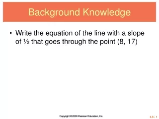
Background Knowledge • Write the equation of the line with a slope of ½ that goes through the point (8, 17)
4.6 Applications and Models of Exponential Growth and Decay The Exponential Growth or Decay Function Growth Function Models Decay Function Models
Exponential Growth or Decay Function Exponential Growth or Decay Function In many situations that occur in ecology, biology, economics, and the social sciences, a quantity changes at a rate proportional to the amount present. In such cases the amount present at time t is a special function of t called an exponential growth or decay function. Let y0 be the amount or number present at time t = 0. Then, under certain conditions, the amount present at any time t is modeled by where k is a constant.
Exponential Growth or Decay Function Think parent functions: When k > 0, the function describes growth; in Section 4.2, we saw examples of exponential growth: compound interest and atmospheric carbon dioxide. When k < 0, the function describes decay; one example of exponential decay is radioactivity.
DETERMINING AN EXPONENTIAL FUNCTION TO MODEL THE INCREASE OF CARBON DIOXIDE Example 1 Find an exponential function that gives the amount of carbon dioxide y inyear t. a. • Equation will take the form • y = y0ekt. We must find the values of y0 and k. • The data began with the year 1990, so to simplify our work we let 1990 correspond to t = 0, 1991 correspond to t = 1, and so on. • Additionally, t=0 corresponds with y=353, so y0 =353 • Calculating k is like finding b in y=mx + b
DETERMINING AN EXPONENTIAL FUNCTION TO MODEL THE INCREASE OF CARBON DIOXIDE Example 1 Find an exponential function that gives the amount of carbon dioxide y inyear t. a. Solution
DETERMINING AN EXPONENTIAL FUNCTION TO MODEL THE INCREASE OF CARBON DIOXIDE Example 1 b. Estimate the year when future levels of carbon dioxide will double the 1951 level of 280 ppm. Solution
FINDING DOUBLING TIME FOR MONEY Example 2 How long will it take for the money in an account that is compounded continuously at 3% interest to double? Solution Continuous compounding formula Let A = 2P and r = .03 Divide by P Take logarithms on both sides.
FINDING DOUBLING TIME FOR MONEY Example 2 How long will it take for the money in an account that is compounded continuously at 3% interest to double? Solution In ex = x Divide by .03 Use a calculator. It will take about 23 yr for the amount to double.
DETERMINING AN EXPONENTIAL FUNCTION TO MODEL POPULATION GROWTH Example 3 According to the U.S. Census Bureau, the world population reached 6 billion people on July 18, 1999, and was growing exponentially. By the end of 2000, the population had grown to 6.079 billion. The projected world population (in billions of people) t years after 2000, is given by the function defined by
DETERMINING AN EXPONENTIAL FUNCTION TO MODEL POPULATION GROWTH Example 3 a. Based on this model, what will the world population be in 2010? Solution Since t = 0 represents the year 2000, in 2010, t would be 2010 – 2000 = 10 yr. We must find (t) when t is 10.
DETERMINING AN EXPONENTIAL FUNCTION TO MODEL POPULATION GROWTH Example 3 b. In what year will the world population reach 7 billion? Solution
DETERMINING AN EXPONENTIAL FUNCTION TO MODEL RADIOACTIVE DECAY Example 4 If 600 g of a radioactive substance are present initially and 3 yr later only 300 g remain, how much of the substance will be present after 6 yr? Solution • Find equation: we use the given values to first find k. • Find amount after t= 6 years.
Half Life Analogous to the idea of doubling time is half-life, the amount of time that it takes for a quantity that decays exponentially to become half its initial amount.
SOLVING A CARBON DATING PROBLEM Example 5 Carbon 14, also known as radiocarbon, is a radioactive form of carbon that is found in all living plants and animals. After a plant or animal dies, the radiocarbon disintegrates. Scientists can determine the age of the remains by comparing the amount of radiocarbon with the amount present in living plants and animals. This technique is called carbon dating. The amount of radiocarbonpresent after t years is given by where y0 is the amount present in living plants and animals.
SOLVING A CARBON DATING PROBLEM Example 5 a. Find the half-life. Solution If y0 is the amount of radiocarbon present in a living thing, then ½ y0 is half this initial amount. Thus, we substitute and solve the given equation for t. Let y = ½ y0 .
SOLVING A CARBON DATING PROBLEM Example 5 b. Charcoal from an ancient fire pit on Java contained ¼ the carbon 14 of a living sample of the same size. Estimate the age of the charcoal. Solution
Stopping Point • Key ideas from today: • Write equations for exponential models in the form • Solving for “k” follows analogous process as solving for “b” in linear models • Close reading of problem to determine if questions asks for us to plug in “x” or “y” value • Use properties of logs and exp to solve equations
MODELING NEWTON’S LAW OF COOLING Example 6 Newton’s law of cooling says that the rate at which a body cools is proportional to the difference C in temperature between the body and the environment around it. The temperature (t) of the body at time t in appropriate units after being introducedinto an environment having constant temperature T0 is where C and k are constants.
MODELING NEWTON’S LAW OF COOLING Example 6 A pot of coffee with a temperature of 100°C is set down in a room with a temperature of 20°C. The coffee cools to 60°C after 1 hr. a. Write an equation to model the data. Solution We must find values for C and k in the formula for cooling. From the given information, when t = 0, T0 = 20, and the temperature of the coffee is (0) = 100. Also, when t = 1, (1) = 60. Substitute the first pair of values into the equation along with T0 =20.
MODELING NEWTON’S LAW OF COOLING Example 6 a. Write an equation to model the data. Solution Given formula Let t = 0, (0) = 100, and T0 = 20. e0 = 1 Subtract 20. Thus,
MODELING NEWTON’S LAW OF COOLING Example 6 Solution Now use the remaining pair of values in this equation to find k. Given formula Let t = 1, (1) = 60. Subtract 20. Divide by 80. Take logarithms on both sides.
MODELING NEWTON’S LAW OF COOLING Example 6 Solution Now use the remaining pair of values in this equation to find k. In ex = x Thus,
MODELING NEWTON’S LAW OF COOLING Example 6 b. Find the temperature after half an hour. Solution To find the temperature after ½ hr, let t = ½ in the model from part (a). Model from part (a) Let t = ½ .
MODELING NEWTON’S LAW OF COOLING Example 6 c. How long will it take for the coffee to cool to 50°C? Solution To find how long it will take for the coffee to cool to 50°C, let (t) = 50. Let (t) = 50. Subtract 20. Divide by 80.
MODELING NEWTON’S LAW OF COOLING Example 6 c. How long will it take for the coffee to cool to 50°C? Solution To find how long it will take for the coffee to cool to 50°C, let (t) = 50. Take logarithms on both sides. In ex = x