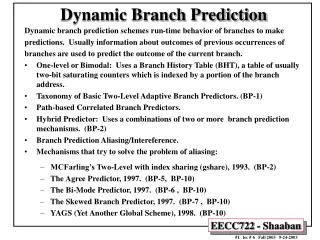
Dynamic Branch Prediction Strategies in Modern Processors
160 likes | 186 Vues
Explore bimodal, global, and local branch prediction techniques. Compare static and dynamic ILP, discussing compiler impact and control hazards in processors. Learn about various branch prediction methods, including 1-bit and 2-bit predictors, correlating predictors, local/global predictors, and tournament predictors used in modern CPUs. Study examples like Alpha, Pentium 4, and Itanium architectures to understand performance trade-offs.

Dynamic Branch Prediction Strategies in Modern Processors
E N D
Presentation Transcript
Lecture 7: Branch prediction • Topics: bimodal, global, local branch prediction • (Sections 2.3-2.6)
Dynamic Vs. Static ILP • Static ILP: • + The compiler finds parallelism no scoreboarding higher clock speeds and lower power + Compiler knows what is next better global schedule - Compiler can not react to dynamic events (cache misses) - Can not re-order instructions unless you provide hardware and extra instructions to detect violations (eats into the low complexity/power argument) - Static branch prediction is poor even statically scheduled processors use hardware branch predictors - Building an optimizing compiler is easier said than done • A comparison of the Alpha, Pentium 4, and Itanium (statically • scheduled IA-64 architecture) shows that the Itanium is not • much better in terms of performance, clock speed or power
Control Hazards • In the 5-stage in-order processor: assume always taken • or assume always not taken; if the branch goes the other • way, squash mis-fetched instructions (momentarily, • forget about branch delay slots) • Modern in-order and out-of-order processors: dynamic • branch prediction; instead of a default not-taken • assumption, either predict not-taken, or predict • taken-to-X, or predict taken-to-Y • Branch predictor: a cache of recent branch outcomes
Pipeline without Branch Predictor PC IF (br) Reg Read Compare Br-target PC + 4 In the 5-stage pipeline, a branch completes in two cycles If the branch went the wrong way, one incorrect instr is fetched One stall cycle per incorrect branch
Pipeline with Branch Predictor PC IF (br) Reg Read Compare Br-target Branch Predictor In the 5-stage pipeline, a branch completes in two cycles If the branch went the wrong way, one incorrect instr is fetched One stall cycle per incorrect branch
Branch Mispredict Penalty • Assume: no data or structural hazards; only control • hazards; every 5th instruction is a branch; branch • predictor accuracy is 90% • Slowdown = 1 / (1 + stalls per instruction) • Stalls per instruction = % branches x %mispreds x penalty • = 20% x 10% x 1 • = 0.02 • Slowdown = 1/1.02 ; if penalty = 20, slowdown = 1/1.4
1-Bit Prediction • For each branch, keep track of what happened last time • and use that outcome as the prediction • What are prediction accuracies for branches 1 and 2 below: • while (1) { • for (i=0;i<10;i++) { branch-1 • … • } • for (j=0;j<20;j++) { branch-2 • … • } • }
2-Bit Prediction • For each branch, maintain a 2-bit saturating counter: • if the branch is taken: counter = min(3,counter+1) • if the branch is not taken: counter = max(0,counter-1) • If (counter >= 2), predict taken, else predict not taken • Advantage: a few atypical branches will not influence the • prediction (a better measure of “the common case”) • Especially useful when multiple branches share the same • counter (some bits of the branch PC are used to index • into the branch predictor) • Can be easily extended to N-bits (in most processors, N=2)
Correlating Predictors • Basic branch prediction: maintain a 2-bit saturating • counter for each entry (or use 10 branch PC bits to index • into one of 1024 counters) – captures the recent • “common case” for each branch • Can we take advantage of additional information? • If a branch recently went 01111, expect 0; if it recently went 11101, expect 1; can we have a separate counter for each case? • If the previous branches went 01, expect 0; if the previous branches went 11, expect 1; can we have a separate counter for each case? Hence, build correlating predictors
Global Predictor A single register that keeps track of recent history for all branches Table of 16K entries of 2-bit saturating counters 00110101 8 bits 6 bits Branch PC Also referred to as a two-level predictor
Local Predictor Also a two-level predictor that only uses local histories at the first level Branch PC Table of 16K entries of 2-bit saturating counters Use 6 bits of branch PC to index into local history table 10110111011001 14-bit history indexes into next level Table of 64 entries of 14-bit histories for a single branch
Local/Global Predictors • Instead of maintaining a counter for each branch to • capture the common case, • Maintain a counter for each branch and surrounding pattern • If the surrounding pattern belongs to the branch being predicted, the predictor is referred to as a local predictor • If the surrounding pattern includes neighboring branches, the predictor is referred to as a global predictor
Tournament Predictors • A local predictor might work well for some branches or • programs, while a global predictor might work well for others • Provide one of each and maintain another predictor to • identify which predictor is best for each branch Alpha 21264: 1K entries in level-1 1K entries in level-2 4K entries 12-bit global history 4K entries Total capacity: ? Local Predictor M U X Global Predictor Branch PC Tournament Predictor Table of 2-bit saturating counters
Branch Target Prediction • In addition to predicting the branch direction, we must • also predict the branch target address • Branch PC indexes into a predictor table; indirect branches • might be problematic • Most common indirect branch: return from a procedure – • can be easily handled with a stack of return addresses
An Out-of-Order Processor Implementation Reorder Buffer (ROB) Branch prediction and instr fetch Instr 1 Instr 2 Instr 3 Instr 4 Instr 5 Instr 6 T1 T2 T3 T4 T5 T6 Register File R1-R32 R1 R1+R2 R2 R1+R3 BEQZ R2 R3 R1+R2 R1 R3+R2 Decode & Rename T1 R1+R2 T2 T1+R3 BEQZ T2 T4 T1+T2 T5 T4+T2 ALU ALU ALU Instr Fetch Queue Results written to ROB and tags broadcast to IQ Issue Queue (IQ)
Title • Bullet