Download
1 / 61
610 likes | 730 Vues
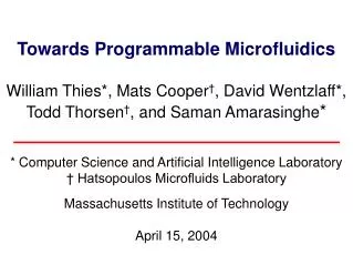
Towards Programmable Microfluidics William Thies*, Mats Cooper † , David Wentzlaff*, Todd Thorsen † , and Saman Amarasinghe *. * Computer Science and Artificial Intelligence Laboratory † Hatsopoulos Microfluids Laboratory Massachusetts Institute of Technology April 15, 2004.

E N D
Towards Programmable MicrofluidicsWilliam Thies*, Mats Cooper†, David Wentzlaff*, Todd Thorsen†, and Saman Amarasinghe* * Computer Science and Artificial Intelligence Laboratory † Hatsopoulos Microfluids Laboratory Massachusetts Institute of Technology April 15, 2004
Microfluidic Chips • Idea: a whole biological lab on a single chip • Input channels for reagants • Chambers for mixing fluids • Actuators for modifying fluids • Temperature - Ultraviolet radiation • Light/dark - Electrophoresis • Sensors for reading properties • Luminescence - Immunosensors • pH - Glucose • Starting to be manufactured and used today • Active area of research
Microfluidic Applications • Biochemistry • Enzymatic assays • The Polymerase Chain Reaction • Nucleic acid arrays • Biomolecular separations • Immunohybridization reactions • Piercing structures for DNA injection
Microfluidic Applications • Biochemistry • Cell biology • Flow cytometry / sorting • Sperm/embryo tools: sperm motility, in vitro fertilization, embryo branding • Force measurements with bending cantilevers • Dialectrophoresis / electrorotation • Impedance monitoring for cell motility and micromotion • Chemical / physical substrate patterning
Microfluidic Applications • Biochemistry • Cell biology • General-Purpose Computing • Compute with fluids • Not our current interest
Microfluidic Applications • Biochemistry • Cell biology • General-Purpose Computing • Summary of Benefits: • High throughput • Small sample volumes • Geometric manipulation • Portable devices • Automatic Control
Our Goal:Provide Abstraction Layers for this Domain • Current interface: gate-level control (e.g., Labview) • New abstraction layers will enable: • Scalability • Currently have 1,000 storage cells, can manage resources by hand • Soon will have 1,000,000: how to manage complexity? • Portability • Hide architecture-specific details from programmer • Same experiment works on successive generations of chips • Modularity • Create reusable components • Enable large and complex procedures • Adaptivity • Use real-time sensor feedback to guide experiment • Adjust procedure to suite field conditions
Our Goal:Provide Abstraction Layers for this Domain • Current interface: gate-level control (e.g., Labview) • New abstraction layers will enable: • Scalability • Currently have 1,000 storage cells, can manage resources by hand • Soon will have 1,000,000: how to manage complexity? • Portability • Hide architecture-specific details from programmer • Same experiment works on successive generations of chips • Modularity • Create reusable components • Enable large and complex procedures • Adaptivity • Use real-time sensor feedback to guide experiment • Adjust procedure to suite field conditions
Our Contributions 1. End-to-end programmable system • General-purpose microfluidic chip • High-level software control 2. Novel mixing algorithms • Mix k fluids in any concentration (± 1/n) • Guarantees minimal number of mixes:O(k log n)
Outline • Introduction • Mixing algorithms • General-purpose microfluidic chip • Portable programming system • Implementation • Related Work • Conclusions
Outline • Introduction • Mixing algorithms • General-purpose microfluidic chip • Portable programming system • Implementation • Related Work • Conclusions
Mixing in Microfluidics • Mixing is fundamental operation of microfluidics • Prepare samples for analysis • Dilute concentrated substances • Control reagant volumes • Important to mix on-chip • Otherwise reagants leave system whenever mix needed • Enables large, self-directing experiments • Analogous to ALU operations on microprocessors
The Mixing Problem • Experiments demand mixing in arbitrary proportions • For example, mix 15% reagant / 85% buffer • Users should operate at this level of abstraction • However, microfluidic hardware lacks arbitrary mixers • Most common model: 1-to-1 mixer • Important optimization questions: • What mixtures are reachable? • How to minimize reagant consumption? • How to minimize number of mixes? 1 unit of A 50% A 50% B 1 unit of mix 1 unit of B
Why Not Binary Search? 0 3/8 1 1/2 1/4 1/2 3/8 5 inputs, 4 mixes
Why Not Binary Search? 0 3/8 1 1/2 3/4 3/8 4 inputs, 3 mixes 1/2 1/4 1/2 3/8 5 inputs, 4 mixes
Mixing Trees • Properties: • Mixing trees are binary trees • Leaf nodes: unit sample of an input fluid • Internal nodes: result of 1-to-1 mix of children • Evaluate from bottom to top • Observation: • # leaf nodes = # internal nodes + 1 (induction on # nodes) • Minimizing mixes and reagant usage is equivalent {(A, ½), (B, ½)} {(A, ¼), (B, 1/8), (C, 5/8)} {(A, ½), (B, ¼), (C, ¼)} {C} {A} {B} {A} {(B, ½), (C, ½)} {C} {B} # reagants used = # mixes + 1
Mixing Trees depth = 0 depth = 1 depth = 2 depth = 3 Theorem: For substance S, let nd denote number of leaf nodes at depth d. Then overall concentration for S is d nd * 2-d Proof: Substance is diluted 2X at each step, and final mixture is sum over all child nodes. {(A, ¼), (B, 1/8), (C, 5/8)} Example: {C} {(A, ½), (B, ¼), (C, ¼)} {C} conc = 2-1 + 2-3 conc = 1/2 + 1/8 {A} {(B, ½), (C, ½)} conc = 5/8 {C} {B}
Reachable Mixtures • Theorem: A mixture is reachable if and only if it can be written: {(S1, p1/2d), (S2, p2/2d), … , (Sk, pk/2d)} • Proof: i pi = 2d Expand to balanced tree S1 S1 S1 S3 S2 S2 S2 S2 p2 p1 p3 Must be mixing tree for mixture Each leaf node contributes 1/2d
Min-Mix Example 2 • Recall example: mixture {(A, 3/8), (B, 5/8)} A=3 B=5 =0011 =0101 B A A B bins 23 = 8 22 = 4 21 = 2 20 = 1 depth = 0 depth = 1 3 mixes Same as optimal depth = 2 depth = 3 c = 2-2 + 2-3 = 1/4 + 1/8 = 3/8 c = 2-1+2-3 = 1/2 + 1/8 = 5/8
Min-Mix Example 2 • Mixture {(A, 5/16), (B, 7/16), (C, 4/16)} A=5 B=7 C=4 =00101 =00111 =00100 A B C B A B bins 24 = 16 23 = 8 22 = 4 21 = 2 20 = 1 C B A B A B • Correctness intuition: put d’th most significant bit at depth d • Can always build tree: induction on # bits at depth d
Min-Mix Algorithm A B C B node buildMixingTree(mixture {(S1, p1/n), ..., (Sk, pk/n)}) { depth = lg(n) bins = new stack[depth+1] for i = 1 to k for j = 0 to depth-1 if (j’th least significant bit of pi =1) { bins[j].push(Si) } return buildMixingHelper(bins, depth) } node buildMixingHelper(stack[] bins, int pow) { if bins[pow].empty() then node child1 = buildMixingHelper(bins, pow-1) node child2 = buildMixingHelper(bins, pow-1) return <child1, child2> as internal node; else return bins[pow].pop() as leaf node; endif } A B bins[4] = { }bins[3] = { }bins[2] = { A, B, C}bins[1] = { B }bins[0] = { A, B } pow43 2 1 0 B C A B A B
Optimality of Min-Mix A • Consider mixture: {(S1, p1/n), … , (Sk, pk/n)} • Number of input samples used = number of bits in representation of inputs • Theorem: this is optimal reagant usage • Implies optimal number of mixes • Proof: otherwise some pi/n is unattainable • Asymptotic reagant usage: O(k lg n) • This is also runtime of Min-Mix (visits nodes once) B C B A B
Supporting Error Tolerances • What if user wants to mix {(A, 1/3), (B, 2/3)}? • Impossible to obtain exactly with 1-to-1 mixer • However, can approximate within tolerance, ± • Error bounds are natural part of all experiments
Supporting Error Tolerances • Method: increase mixing depth d until some mix p1/2d … pk/2d falls within desired ranges • Example: mix {(A, 1/3), (B, 1/3), (C, 1/3)} ± 0.05? • Each substance should fall in range [0.23, 0.43] Depth Concentrations 1 0.5 - Out of range 2 0.25,0.5,0.75 - In range, but infeasible: 0.25 + 0.25 + 0.25 < 1 3 …, 0.25, 0.375, … - In range and feasible: 0.25 + 0.375 + 0.375 = 1 - Could be multiple solutions; we choose greedily 0 1
Outline • Introduction • Mixing algorithms • General-purpose microfluidic chip • Portable programming system • Implementation • Related Work • Conclusions
What Does General-Purpose Mean? • Computing: Turing Machine • Implementation parameter: memory size • Microfluidics: “Universal Fluidic Machine” • Implementation parameters: • memory size precision sensors/agitators
Our General-Purpose Chip (April 2004) 5 mm Control layer Flow layer
Our General-Purpose Chip (April 2004) 5 mm Multiplexor Purge Out Control layer Flow layer • 8 storage cells • Individually addressable • 9 picoliters each Control ports Mixer Storage Cells • Rotary mixer (Quake et al.) Wash In • Input / Output • Can also add I/O ports to storage cells
Chip-Level Operations A B • All operations are “pushed” by input, flow to purge out • Extra inputs / outputs attached to storage cells • Basic operations: • storage output • storage mixer • mixer storage • Due to precision limits, output of mixer only fillsone storage cell • storage storage is“mix 2 of same fluid and store” Purge Out Wash In
Outline • Introduction • Mixing algorithms • General-purpose microfluidic chip • Portable programming system • Implementation • Related Work • Conclusions
A Portable Machine Language (PML) • C is PML for von-Neumann machines • Hides idiosyncratic differences • Exposes important properties • Enables portability • Things to virtualize in microfluidic realm: • # of chambers, pipes, mixing reservoirs, etc. • Location of fluids on the chip • Precision of mixing and routing hardware • Timing of events • Our solution: Lava • A Java library with first-class Fluid objects • Virtualizes basic resources • Provides native hooks for common agitators / sensors
Example: Recursive Descent Search • Goal: find ratio of two fluids with highest activity • Common question in biology • Modeling activators / inhibitors • Understanding signaling pathways • Drug discovery • Method: zoom in on area of interest set range = [0,1] for each round { for each point p in range { measure activity at p } adjust range around highest activity } report range and activity 1 2 3 Round: Range:
Example: Recursive Descent Search interface SimpleEngine extends FluidEngine { Fluid input(Integer i); // require array of fluid inputs Double luminescence(Fluid f); // require luminescence camera } class RecursiveDescent { public static void main(String[] args) { SimpleEngine engine = (SimpleEngine) // build engine for interface EngineFactory.buildEngine("SimpleEngine", MY_BACKEND); run(engine); } static void run(SimpleEngine engine) { … } }
Example: Recursive Descent Search static void run(SimpleEngine engine) { Fluid A = engine.input(new Integer(0)); // input Fluids Fluid B = engine.input(new Integer(1)); double center = 0.5, radius = 0.5; // set range of interest double act, bestActivity = -1; for (int i=0; i<ROUNDS; i++) { // repeat a number of rounds int bestJ = 0; for (int j=0; j<10; j++) { // try 10 samples double target = center+radius*(1-2*(double)j/10); Fluid f = engine.mix(A, target, B, 1-target); // prepare mixture engine.waitFor(30); act = engine.luminescence(f).doubleValue(); // measure activity if (act > bestActivity) { bestActivity = act; bestJ = j; // remember highest activity }} center = center+radius*(1-2*(double)bestJ/10); // zoom in on highest activity radius = radius / 2; } System.out.println("Highest activity at: " + center); }
Providing Digital Abstraction • Challenge: Fluid variables used multiple times • But once a fluid is used on-chip, it is gone! • This is a lossy system • Need to provide some notion of GAIN
Providing Digital Abstraction • Challenge: Fluid variables used multiple times • Solution: re-generate fluids on demand • Lava traces history for computing each Fluid • Current model: stateless mixing, native functions • If unavailable fluid referenced, re-evaluate history • Optimizations • Lazy evaluation • Evaluate in order that minimizes temporaries input (0) input (0) heat(10) mix mix wait(30) input (1)
Outline • Introduction • Mixing algorithms • General-purpose microfluidic chip • Portable programming system • Implementation • Related Work • Conclusions
Implementation Status (April 2004) • Prototype chip fabricated • Demonstrated I/O, moving fluids, mixing • Current focus: • Robustness • Air bubbles • Diffusion • Calibration • Need to determinetiming for automatic control
Fabrication Process (Quake et al.) Control Layer 0. Start with mask of channels Flow Layer
Fabrication Process (Quake et al.) Control Layer 1. Deposit pattern on silicon wafer Flow Layer
Fabrication Process (Quake et al.) Control Layer 2. Pour PDMS over mold - polydimexylsiloxane: “soft lithography” Thick layer (poured) Thin layer (spin-coated) Flow Layer
Fabrication Process (Quake et al.) Control Layer 3. Bake at 80° C(primary cure), then release PDMS from mold Flow Layer
Fabrication Process (Quake et al.) Control Layer 4a. Punch hole in control channel4b. Attach flow layer to glass slide Flow Layer
Fabrication Process (Quake et al.) Control Layer 5. Align flow layer over control layer Flow Layer
Fabrication Process (Quake et al.) Control Layer 6. Bake at 80° C (secondary cure) Flow Layer
Fabrication Process (Quake et al.) 7. When pressure is high, controlchannel pinches flow channel toform a valve Control Layer pressure actuator Flow Layer
Making a Multiplexor (Thorsen et al.) flow layer control layer Bit 2 Bit 1 Bit 0 1 1 1 0 0 0 Output 7 • Control lines can cross flow lines • - Only thick parts make valves Output 6 Output 5 Input Output 4 • Logic is not • complimentary • To control n flow lines, • need 2 log2 n control lines Output 3 Output 2 Output 1 Output 0
Making a Multiplexor (Thorsen et al.) flow layer control layer Bit 2 Bit 1 Bit 0 1 1 1 0 0 0 Output 7 • Control lines can cross flow lines • - Only thick parts make valves Output 6 Output 5 Input Output 4 • Logic is not • complimentary • To control n flow lines, • need 2 log2 n control lines Output 3 Output 2 Output 1 Output 0 Example: select 3 = 011
Making a Multiplexor (Thorsen et al.) flow layer control layer Bit 2 Bit 1 Bit 0 1 1 1 0 0 0 Output 7 • Control lines can cross flow lines • - Only thick parts make valves Output 6 Output 5 Input Output 4 • Logic is not • complimentary • To control n flow lines, • need 2 log2 n control lines Output 3 Output 2 Output 1 Output 0 Example: select 3 = 011