Model Validation in Discrete Event Simulation Process
360 likes | 401 Vues
Understand the stages of validation in simulation modeling process to ensure accuracy and reliability. Includes design, implementation, verification, and validation phases.

Model Validation in Discrete Event Simulation Process
E N D
Presentation Transcript
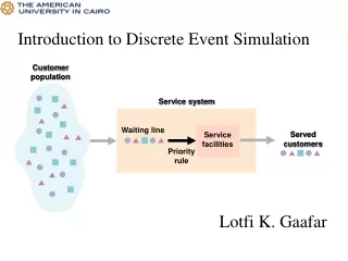
Discrete Event Simulation - 7 Model Validation
Discrete Event Simulation - 7 What do we mean by "Model Validation"? There is no way in which we can PROVE that our simulator (model) matches reality - all we could prove is that it does NOT. What are the stages that we go through in order to determine that the simulator is - as far as we can tell - acceptable?
Discrete Event Simulation - 7 • Design Phase. This consists of using A) our intuitive and mathematical understanding of the process we are trying to model; B) our experience in designing computer models of reality; C) techniques of software engineering developed to aid the transition from A) and B) to a codable specification. These might simply include modular decomposition and top-down design, or more sophisticated specification languages and environments.
Discrete Event Simulation - 7 • Validation of Design A) Conceptual Phase: determine the logical flow of the system, and formulate the relationships between the various subsystems. Identify the factors likely to influence the performance of the model and decide how you will track them. Validation by review: have a third party examine the design in detail. Validation by tracing from output to input: this is just the opposite from the usual direction, and might indicate gaps and misunderstandings.
Discrete Event Simulation - 7 • Validation of Design B) Implementation Phase: selecting procedures for the model; coding the model; using the model. Validation by checkpoints and milestones: at the end of the model design phase; at the end of the implementation of each module; at the integration of two or more modules. The latter two require that individual module tests have been identified and designed, and that the flow of information between modules can be examined in detail. This blends into the next phase...
Discrete Event Simulation - 7 • Verification Phase. Does the system that has been coded meet the specifications? At this point, the design might well be "wrong", and this phase is not meant to catch design mistakes. It should catch any deviations of the actual implementation from the design specifications. How: code walk-throughs, careful tracing of module interfaces and module dependencies, tests that were designed at specification time for this purpose.
Discrete Event Simulation - 7 • Validation Phase At this point we have a running program that we believe satisfies the design specifications and - because the design was achieved by people with experience in designing such simulation models using some design validation methods - is probably close enough to reality so that its inputs and outputs can be meaningfully compared with those of the "real thing". We want to establish that the model is an "adequately accurate" representation of the reality we are interesting in modeling. If this cannot be established, our model will be useless for both explanation and prediction - both of which are goals of "good models".
Discrete Event Simulation - 7 • What does Validation Consist of? • A) Comparison of results of simulation model with historical data; • B) Use of the simulation model to predict behavior of the real system, and compare prediction with actual behavior. • Both of these methods are standard when it comes to validating a physical theory: the theory must not contradict any "well-known facts"; it must provide new predictions (not available through established theory) that are subject to falsification by experiment.
Discrete Event Simulation - 7 • How do you determine that the system has been validated? • Even in Physics, theoretical predictions usually do not match experimental results exactly. • Solution: run statistical tests, until you can conclude, from statistical considerations, that the probability of some competing explanation being true is smaller than a preassigned quantity. • This means that the system must be designed for multiple controlled observations and the collection of all appropriate data (= measures of performance).
Discrete Event Simulation - 7 Definition: Simulation Run. This is an uninterrupted recording of the simulation system's performance given a specified combination of controllable variables: range of values, values of some parameter, queue arrival distributions, etc.
Discrete Event Simulation - 7 Definition: Simulation Duplication. This is a recording of the simulation system's performance given the same or replicated conditions and/or combinations, but with different random variates. This is also related to "regression testing": a correct model (or piece of software) must satisfy certain input/output relations. Any time the software is modified it must pass all the old tests; if it is "improved", it must pass all the old tests plus appropriate new ones.
Discrete Event Simulation - 7 Definition: Simulation Observation. This is a simulation run or a segment of a simulation run that is sufficient for estimating the value of each of the performance measures.
Discrete Event Simulation - 7 Definition: Steady State or Stable State. This state of a simulation system is achieved when successive system performance measurements are statistically indistinguishable - the second one provides no new information about the future behavior of the system. Steady State corresponds, for example, to the constant solution of a differential equation. A Stable Steady State corresponds to a stable constant solution or, more likely, to an asymptotically stable one.
Discrete Event Simulation - 7 How do we identify a steady state of some performance measure? By deciding on a "small" positive value, say e, and deciding that we have reached steady state when, over a "long" period of time, the performance measure (or some appropriate function of it) has remained within ±e of some value. "small" and "long" are terms that are meaningful only in the context of the particular model being studied. It may also be possible to actually predict, from the model, the constant value.
Discrete Event Simulation - 7 Definition: Transient State. The time (and set of performance measurements) that correspond to the initial conditions becoming insignificant to the future behavior of the system. Some systems may have no Steady State, so that no termination for a Transient State could be identified.
Discrete Event Simulation - 7 Most simulations appear to be interested in examining the steady state behavior. This is appropriate under some conditions - and in the case where modeling based on discrete queueing theory is being used: most such queueing theory results depend on our being able to obtain steady state predictions. There are other situations where the transient state may be the most important, since that is where system queues (or buffers) might be overloaded. The "usual solution" is to provide enough system capacity to handle "most" transients. This requires that we find good prediction for the size of all "transients" in the measures of performance.
Discrete Event Simulation - 7 A further problem with transients is that the actual behavior depends on the exact initial conditions of the system. As it turns out, some systems may have very complex initial conditions - possibly extending over long periods of time. Some systems may exhibit very complex behavior - so that some initial conditions will tend to one steady state (or, more generally, an "attractor" which may exhibit a very complex geometry) while others will lead to another all without varying the parameters of the system. These are so-called bistable (or multistable) systems.
Discrete Event Simulation - 7 Studying transient behavior will thus require a large number of runs; a possibly complex geometric analysis of the "phase-space" of the system; the ability to describe and set arbitrary initial conditions for the system; and sophisticated statistical techniques to determine means, variances and other statistics of the relevant performance measures. If one wishes to avoid dealing with transient behavior, one must be able to specify initial conditions near steady state: this may require being able to "load the model" with a specific history.
Discrete Event Simulation - 7 In simple cases this might just mean deferring data collection for a period of time; in others it might mean that consistent performance measure values have to be synthesized over a long enough time period and that these measures have to be "inserted" into the behavior of the model.
Discrete Event Simulation - 7 What is Validation - again. How accurately is the simulation model representing the actual physical system being simulated? Several terms have been introduced, corresponding to techniques that help in answering this question. One must always remember that there is no way to prove that the model is a faithful reproduction of reality. All we can prove is that it is not. But we might be able to set up enough different experiments so that passing of all the experimental tests will allow us to conclude that the probability the model is inaccurate is very small.
Discrete Event Simulation - 7 Internal Validity. This is affected by variability due to internal "noise" effects: stochastic models with high variance due to internal processing will provide outputs whose analysis may not be very useful: are the changes in the outputs due to the model or to incidentals of the implementation? (e.g., numerical approximation errors due to the presence of singularities in some of the functions used)
Discrete Event Simulation - 7 Face Validity: Compare model output results with actual output results of the real system. Variable-Parameter Validity: compare sensitivity to small changes in internal parameters or initial values with historical data. Compare model dependencies with historical data, looking for the same dependencies. Event or Time-Series Validity: does the model predict observable events, event patterns and variations in output variables?
Discrete Event Simulation - 7 Some Ideas about Data Collection (Sampling). The text discusses ways to determine whether the data collected are correlated or not. One would like to obtain stochastically independent data sets, or one would like, at least, to determine the level of correlation between data sets. This is where the covariance - or the coefficient of correlation - comes in, since it allows us to determine something about dependence.
Discrete Event Simulation - 7 Repetition: how many runs and how long should they be? Blocking: how do we avoid the contributions of transient periods (this assumes we are interested in steady-state behavior).
Discrete Event Simulation - 7 We can attempt to determine whether two runs are independent in the following way. Let the xi denote individual observations, n the number of observations. Let the average estimated performance measure be If each if the xi is independent, the confidence of this performance measure is just the estimate of the variance
Discrete Event Simulation - 7 If {xi; i = 1,…,n/2}, {yi; i = 1,…,n/2} are two sets of observations, we can try to find out whether they are correlated. We observe that the mean of the union of the two sets can be written as The variance can be written as Where a is the replication correlation coefficient. The formula can be derived through the following observations:
Discrete Event Simulation - 7 Where and a is the coefficient of correlation. Using this in the original formula, and under the assumption that the two samples come from the same population (equal population variance): Since the variance of the means is given by the population variance divided by sample size, we have:
Discrete Event Simulation - 7 If two runs (replications) are independent, then a=0, since they must behave exactly as one run of twice the length (i.e. n). We now have a way to test whether two successive runs are correlated or not.
Discrete Event Simulation - 7 To see what negatively correlated runs can do, assume we have obtained the following set of observations: X = [.3211106933, .3436330737, .4742561436, .5584587190, .7467538305, .3206222209e-1, .7229741218, .6043056139, .7455800374, .2598119527, .3100754872, .7971794905, .3916959416e-1, .8843057167e-1, .9604988341, .8129204579, .4537470195, .6440313953, .9206249473, .9510535301] from a uniform random number generator. The "complementary" set (1 - r, for each r in the first set) is Y = [.6788893067, .6563669263, .5257438564, .4415412810, .2532461695, .9679377779, .2770258782, .3956943861, .2544199626, .7401880473, .6899245128, .2028205095, .9608304058, .9115694283, .395011659e-1, .1870795421, .5462529805, .3559686047, .793750527e-1, .489464699e-1]
Discrete Event Simulation - 7 The coefficient of correlation is given by Maple V as a = describe[covariance](X,Y)/sqrt(describe[variance](X)* describe[variance](Y)) = -.9999999996 Very close to -1. What is the actual variance for the joint population? The formula we use must lead us to a run of 20 items where each item is the mean of the corresponding two items in the separate populations. But (xi + yi)/2 = (ri + (1 - ri))/2 = 1/2, m = 1/2 and the sample variance is given by Negative correlation leads to a smaller variance than independence, while positive correlation leads to a larger variance.
Discrete Event Simulation - 7 If we want to estimate means and variances of different runs - i.e. runs with different conditions. We have estimated sample means and variances to be The mean and variance of the difference are Where a is the usual coefficient of correlation. The difference in the formula is due to the difference for the statistics - rather than the sum. It is immediate to see that positively correlated runs will diminish the variance of the difference. To check whether positively correlated runs will make the variance small.
Discrete Event Simulation - 7 One of the problems is the elimination of transient information. In this case it will be advisable to have long runs, in which the early part has been ignored. One method that helps find out a reasonable length for the run involves computation of the autocorrelation function. This is defined as: Where xt is an observation at time t; m is the mean of the observations and s2 is their variance. Note that D = 0, gives that a(0) = 1.
Discrete Event Simulation - 7 The sample mean is computed in the usual manner, while the variance of the sample means is given by the formula Notice that a(D) = 0 for all D > 0 implies that the observations are independent - and this is reflected in the formula. Correlated observations will thus enlarge the variance of the sample means.
Discrete Event Simulation - 7 The Blocking Method. This simply consists of A) Wait until transients are over; B) collect successive blocks of observations of length k is such a way that the "block means" satisfy independence conditions. C) Use the block means as “observations” to compute the sample mean and the variance of the sample means. The independence conditions can be checked via any of the methods already mentioned.