SQL Recap and Examples: Group By, Having, and Tuple Calculus
280 likes | 389 Vues
Covering SQL concepts like group by, having, and advanced tuple calculus, with examples illustrating these topics.

SQL Recap and Examples: Group By, Having, and Tuple Calculus
E N D
Presentation Transcript
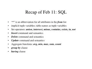
Recap of Feb 11: SQL • “*” is an abbreviation for all attributes in the from list • implicit tuple variables; table names as tuple variables • Set operators: union, intersect, minus, contains, exists, in, not • Insert command and semantics • Delete command and semantics • Update command and semantics • Aggregate functions: avg, min, max, sum, count • group by clause • having clause
SQL: Multiple Group Bys Example: using relation emp(ss#, ename, dept, cat, sal) Count the employees and average monthly salary for each employee category in each department select dept, cat, count(*), avg(sal)/12 from emp group by dept, cat
Select … from emp group by cat Select … from emp group by dept SQL: Multiple Group Bys
SQL: Multiple Group By Select … from emp group by dname, cat note that some dname/cat groups are empty.
SQL: Examples on Having Find the average salary of employees under 30 for each department with more than 10 such employees select dname, avg(sal) from emp where age<30 (employee age under 30) group by dname (group by department) having 10<count(*) (group size > 10)
SQL: Examples on Having Find the average salary of employees under 30 for each department with more than 10 employees select e.dname, avg(e.sal) from emp e where e.age<30 (employee age under 30) group by e.dname (group by department) having 10<any (select count(ee.ename) (number of employees in group) from emp ee where ee.dname=e.dname) (… from the same dept as e) (why is this query different from the previous one?)
SQL: Examples on Having Find categories of employees whose average salary exceeds that of programmers select cat, avg(sal) from emp group by cat having avg(sal)> (select avg(sal) from emp where cat=“programmer”)
SQL: Examples on Having Find all departments with at least two clerks select dname from emp where job=“clerk” group by dname having count(*) >= 2
SQL: Examples Find the names of sailors with the highest rating select sname from sailors where rating = (select max(rating) from sailors)
SQL: Examples For each boat, find the number of sailors of rating >7 who have reserved this boat select bid, bname, count(s.sid) from sailors s, boats b, reserve r where s.sid=r.sid and r.bid=b.bid and rating>7 group by b.bid
SQL: Examples For each red boat, find the number of sailors who have reserved this boat select bid, bname, count(s.sid) from sailors s, boats b, reserve r where s.sid=r.sid and r.bid=b.bid group by b.bid having colour=“red”
SQL: Examples Difference between the last two queries? • First one gave a qualification on the tuples (take all tuples of the multijoin discard tuples that do not fulfill ratings>7 then group them by boat id then find the cardinality of each group) • Second one gave a qualification for the groups (take all tuples of the multijoin group them by boat id discard groups representing boats that are non-red find the cardinality of remaining groups)
And Now, For SomethingCompletely Different... • The recent SQL material largely covers chapter 4, at least sections 4.1 through 4.6 and some of 4.9. • Earlier we examined Relational Algebra, covering sections 3.1 through 3.3 • Now we leave chapter 4 and head back to examine sections 3.6 and 3.7, covering Relational Calculi • based upon predicate calculus • non-procedural query languages (descriptive rather than prescriptive) • we will examine two relational calculi: tuple calculus and domain calculus
Tuple Calculus Query: {t | P(t)} P: is a predicate associated with some relation R t: is a tuple variable ranging over the relation R t[A]: is the value of attribute A in tuple t • students in CMSC 424 • {t | t enroll t[course#] = CMSC424} • students in CMSC 424 conforming with the CMSC-420 prerequisite • {t | t enroll s enroll t[course#] = CMSC424 s[course#] = CMSC420 t[ss#] = s[ss#]}
Tuple Calculus • Quantifiers and free variables • , quantify the variables following them, binding them to some value. (in the previous slide, s was bound by ) • A tuple variable that is not quantified by or is called a free variable. (in the previous slide, t was a free variable) • Atoms • R(t) where t is a tuple variable • t[x] s[y] where t,s are tuple variables and {, , , , , }
Tuple Calculus • Formulas • an Atom is a Formula • If P and Q are Formulas, then so are (P), P, PQ, PQ, and PQ • If P(t) is a Formula, then so are t P(t) andt P(t) • Equivalences • (P Q) P Q • (P Q) P Q • t P(t) (t ( P(t))) • t P(t) ( t ( P(t)))
Tuple Calculus • Safety • Math is too powerful; we can easily phrase expressions that describe infinite sets {t | t enroll} • These expressions are called unsafe • When we are dealing with finite sets, unsafe expressions happen in expressions that involve negation () • We can avoid this problem by using an entirely positive (non-negated) scope as the first operand of any conjunction where we use negation. The first operand establishes the scope and the second one filters the established scope. {t | t enroll t[course#] CMSC-420}
Domain Calculus • Another form of relational calculus • Uses domain variables that take values from an attribute’s domain, rather than values representing an entire tuple • Closely related to tuple calculus • Domain Calculus serves as the theoretical basis for the query language QBE, just as the relational algebra we examined earlier forms the basis for SQL • Expressions are of the form: {< x1, x2, x3, ..., xn> | P( x1, x2, x3, ..., xn) }
Domain Calculus • Atoms • < x1, x2, x3, ..., xn> R • x y where x,y are domain variables and {, , , , , } • x c where c is a constant • Formulas • an atom is a formula • If P and Q are formulas, then so are (P), P, PQ, PQ, and PQ • If P(x) is a formula and x is a domain variable, then x P(x) andx P(x) are also formulas
Domain Calculus • Queries are of the form: {< x1, x2, x3, ..., xn> | P( x1, x2, x3, ..., xn) } • Examples {<ss#, course#, semester> | Enroll(ss#, course#, semester)} {<x, y, z> | Enroll(x, y, z) y = CMSC-424}
Reductions of Relational Algebra and Calculi • Relational Algebra (sections 3.2-3.5), Tuple Calculus (section 3.6), and Domain Calculus (section 3.7) can be reduced to each other: they have equivalent expressive power. For every expression in one, we can compute an equivalent expression in the others.
Functional Dependencies • Important concept in differentiating good database designs from bad ones • FD is a generalization of the notion of keys • An FD is a set of attributes whose values uniquely determine the values of the remaining attributes. Emp(eno, ename, sal) key FDs: eno => ename Dept(dno, dname, floor) eno => sal Works-in(eno,dno, hours) (eno,dno) => hours dno => dname dno => floor
Functional Dependencies • If R and R, then => holds in the extension r(R) of R iff for any pair t1 and t2 tuples of r(R) such that t1()=t2() , then it is also true that t1() = t2() • We can use FDs as • constraints we wish to enforce (e.g., keys) • for checking to see if the FDs are satisfied within the database R( A B C D) 1 1 1 1 A => B satisfied? no 1 2 1 2 A => C satisfied? yes 2 2 2 2 C => A satisfied? no 2 3 2 3 AB => D satisfied? yes 3 3 2 4
Functional Dependencies • Trivial dependencies: => => if • Closure • we need to consider all FDs • some are implied by others; e.g., FDs are transitive; if A=>B and B=>C, then A=>C • Given F = set of FDs, we want to find F’ (the closure of all FDs logically implied by F)
Armstrong’s Axioms • Reflexivity if then => • Augmentation if => then • Transitivity if => and => then => Armstrong’s Axioms can be used to derive three additional useful rules: • Union rule if => and => then => • Decomposition rule if => then => and => • Pseudotransitivity rule if => and => then =>
FD Example R(A, B, C, G, H, I) F=( A=>B A=>C CG => H CG => I B => H ) F+=( A => H transitivity: A => B => H CG => HI union rule: CG => H, CG => I AG => I augmentation: A=> C, AG => CG => I AG => H ) augmentation: A=> C, AG => CG => H
Closure of Attribute Sets • Useful to test if an attribute set is a superkey • the closure + of a set of attributes under F is the set of all attributes that are functionally determined by • there is an algorithm to compute the closure R(A, B, C, G, H, I) F=(A=>B, A=>C, CG => H, CG => I, B => H ) Example: Algorithm to compute (AG)+ starts with result=(AG) A=>B expands result=(AGB) A=>C expands result=(AGBC) CG=>H expands result=(AGBCH) CG=>I expands result=(AGBCHI) B=>H causes no more expansion
Uses of Attribute Closure • Testing for superkey • to test if is a superkey, compute + and determine if + contains all attributes of R • Testing functional dependencies • to check if a functional dependency => holds, (is in F+) just check to see if + • in other words, we compute + using attribute closure, and then check if the result contains . • Simple, cheap, and useful test.